Programming Projects for Advanced Beginners #4: Photomosaics
03 Nov 2018
This is a programming project for Advanced Beginners. If you’ve completed all the introductory programming tutorials you can find and want to sharpen your skills on something bigger, this project is for you. You’ll get thrown in at the deep end. But you’ll also get gentle reminders on how to swim, as well as some new tips on swimming best practices. You can do it using any programming language you like, and if you get stuck I’ve written some example code that you can take inspiration from.
NEW
Subscribe to my new "Programming Feedback for Advanced Beginners"
newsletter to receive concise weekly emails containing specific,
real-world ways to make your code cleaner and more professional.
Each week I review code sent to me by one of my readers. I highlight
the things that I like, discuss the
things that I think could be better, and offer suggestions for how
the author could make their code cleaner and easier to work with.
Subscribe now to receive these invaluable improvements in your inbox
every week, completely free.
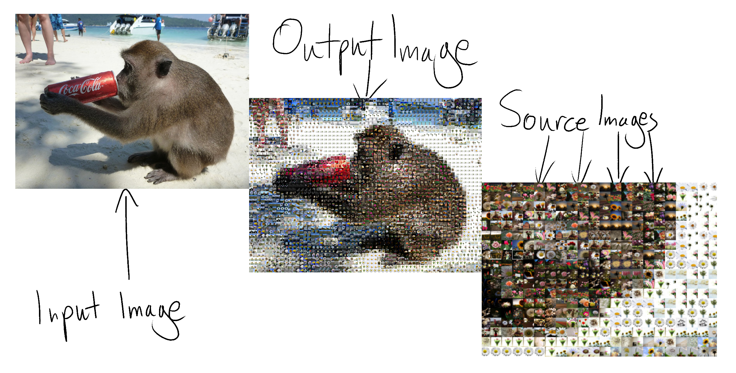
You may have come across photomosaics before - big pictures built out of thousands of other tiny pictures. In this project you’re going to build a photomosaic creator.
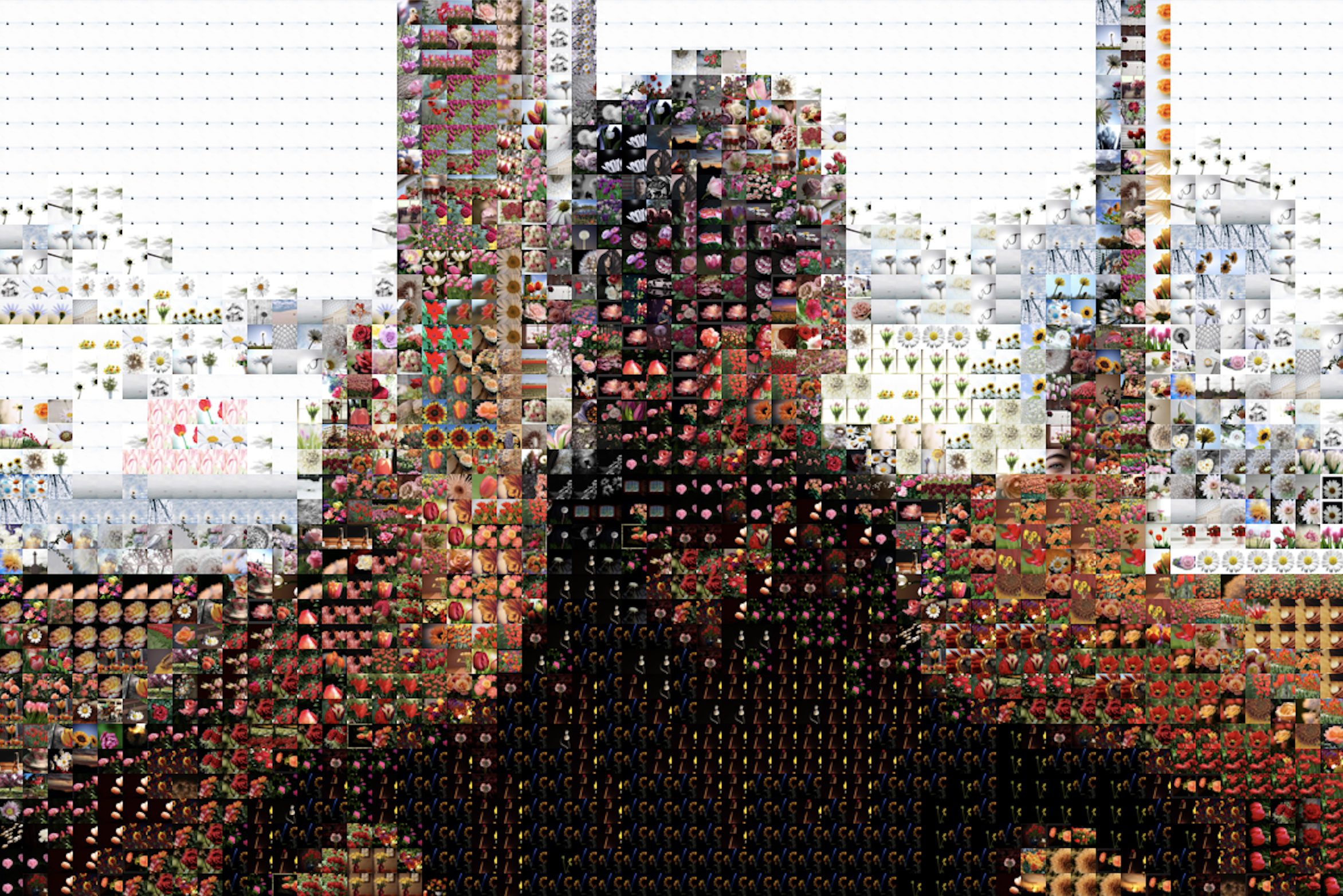
Unlike most other advanced beginner projects, a photomosaic creator is an extremely useful and practical tool. You can use it to mass-produce heartfelt, cheap, and easy presents for your friends and family. You can use it to create deep art with hidden meaning. You can make a picture of a delightful puppy out of thousands of pictures of murderous sharks, or a picture of a murderous shark out of thousands of pictures of delightful puppies. What do these works mean? Are they anti-capitalist, or pro? You don’t even have to decide.
The Plan
As in all Programming Projects for Advanced Beginners, we’ll build our program out of small components and intermediate milestones that we can test and verify individually. If small components and intermediate milestones are new concepts to you then you can either take a quick detour through my previous programming projects (here’s #1, #2 and #3), or push ahead with this project and pick things up as you go along.
We’ll start by sketching out a brief plan, and then get right on to coding. Before reading any further, spend a few minutes drawing up a plan of your own. What should we work on first? What about after that? What sub-problems will we need to solve? What intermediate milestones can we use to make sure we’re heading in the right direction? How can we test each milestone individually, even if we haven’t yet finished the entire program?
Take some time to think about the problem and devise your own plan before you continue - this is an important skill to develop.
My plan
Before I describe the plan that I came up with, let’s agree on some terminology to refer to the different pieces of our project. These aren’t official, technical definitions - they’re just names that I’ve made up for this project.
- Input image - the original image that we are going to recreate
- Output image - the finished photomosaic version of the input image
- Source images - the smaller images that the output image is made out of
We’ll also talk a lot about image processing libraries. An image processing library is a pre-written set of tools for loading and working with images. Almost every programming language has one (or several); have a look at section 1 of my ASCII art project for more advice on getting one set up.
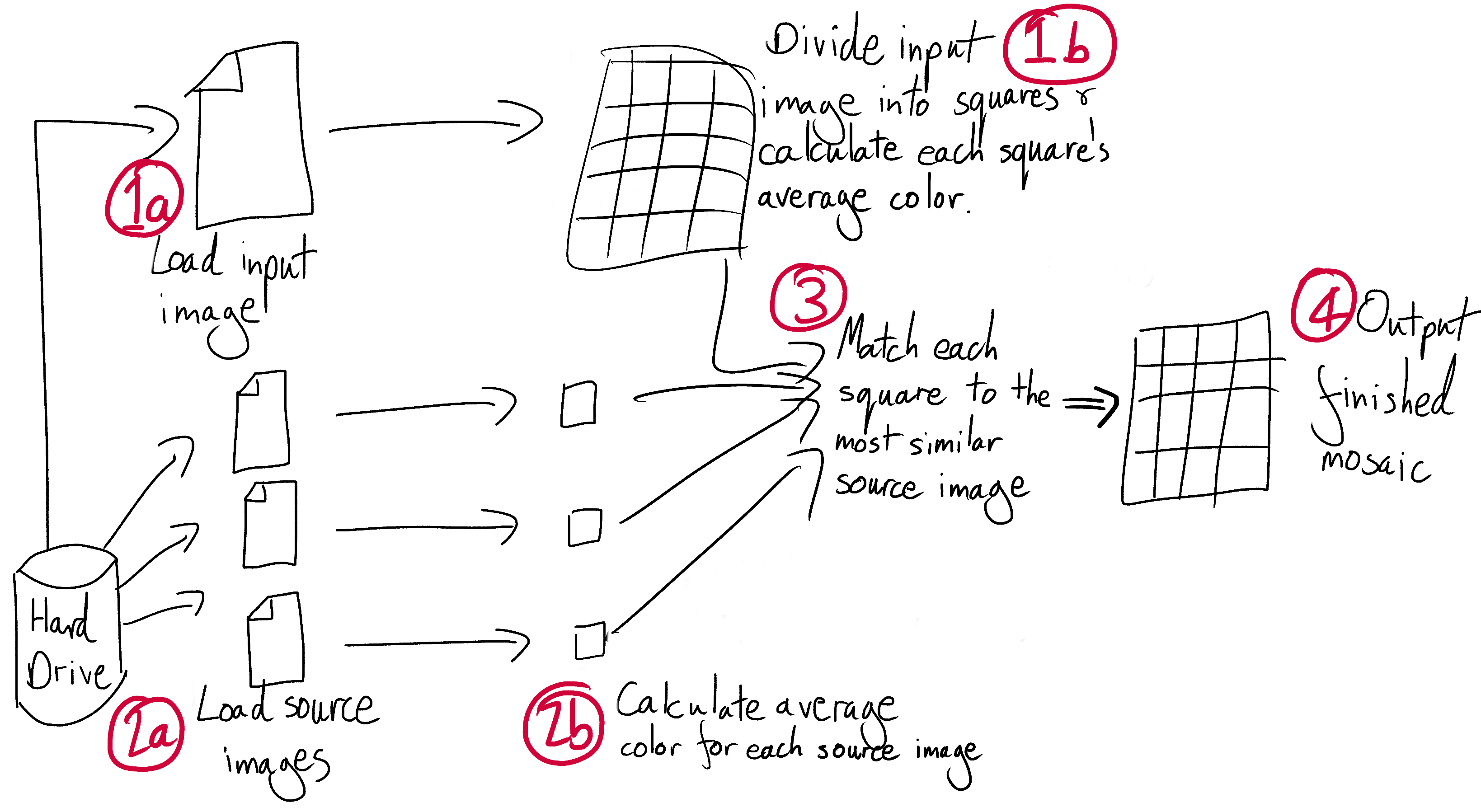
For my plan I’ve come up with 7 steps:
1a. Use an image processing library to load an input image into your code. Paste your input image into a new output image. Mess around with it - rotate it, resize it, add a caption, and generally get familiar with your image processing library.
1b. Divide the input image into squares, and calculate the average color of each square
1c. A quick diversion - create an output image out of squares of these average colors. This will be a pixellated version of your input image!
2a. Find an initial set of 100 source images. Write a script that crops them all to squares and saves the cropped versions
2b. Calculate the average color of each source image
- For each section of the input image, find the source image with the closest average color
- Paste each of these source images into the output image in the appropriate location. You have a photomosaic!
Here’s a map of the system we’re aiming for:
We may change direction or get a little lost on the way, but at least we now have a solid idea of where we’re heading. I’ll race you there.
(note that this is not actually a race and you should take as much time as you need)
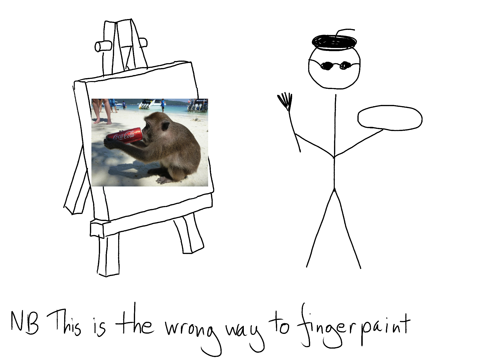
1a. Load the input image
Start by using your image processing library to load your input image. Make sure that the library is working correctly and start to get acquainted with its functionality and documentation. Experiment a bit. For example:
- Print the height and width of your image
- Shrink your image by 50%
- Rotate your image 180 degrees
- Draw a big red rectangle in the middle of your image
- Apply some Instagram-style filters
- Make an artistic collage of several different images
Express yourself. Think of this as finger-painting in code. There’s no right or wrong way to finger-paint.
1b. Divide and calculate
Next, divide your image up into squares, around 50x50 pixels in size, and for each square calculate the average color. Keep in mind that we’re going to reuse this code for calculating the average color of our source images too.
Image processing libraries load images as an array (or sometimes an “array of arrays”) of pixels. Each pixel is represented as an RGB tuple, a group of 3 numbers between 0 and 255 that represent the amount of red, green and blue in the pixel. Red, green and blue are the primary colors of light, and in the right proportions can be combined to create every single other color in existence.
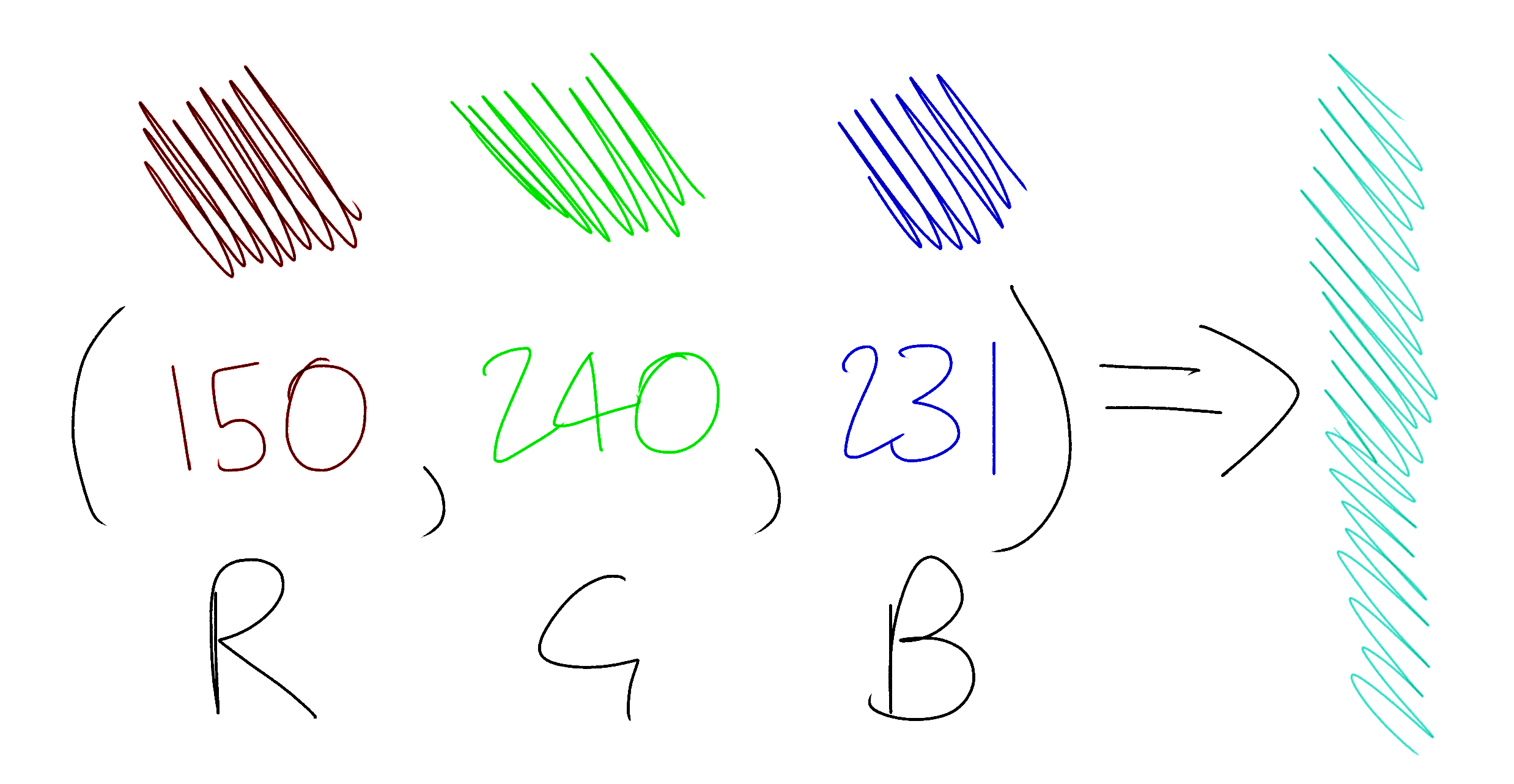
The average color of an image section is simply the combination of the average red, green and blue values of its pixels. For example, if your pixels are:
[
   (100, 71, 150),
   (50, 71, 200),
   (0, 71, 100),
]
then their average color is:
red = (100 + 50 + 0) / 3 = 50
green = (71 + 71 + 71) / 3 = 71
blue = (150 + 200 + 100) / 3 = 150

=> (50, 71, 150)
For more examples of working with pixels, arrays of arrays, and RGB values, see section 1 of my ASCII art project.
For now, don’t worry about doing anything with the average colors that you calculate - just print them to the terminal and make sure they look plausible. At the very least, are all the numbers between 0 and 255?
1c. Pixellate
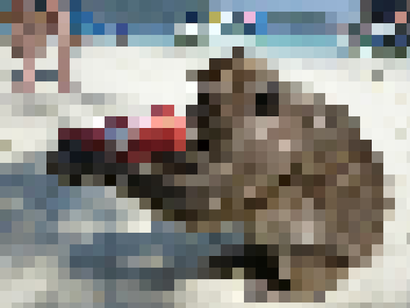
This step isn’t part of the main project, but it is well worth a quick detour. Take the average colors that you just calculated and construct a new image out of squares of these average colors. This output image should look like a pixellated version of your input.
Experiment with changing the size of the squares. What effect does this have?
2a. Crop the source images
Now we’ll turn our attention to our source images. These are the small pictures that our larger output image will be built out of.
First, find an initial set of source images. A copy of the Photos directory on your computer is perfect. Alternatively Kaggle, a machine learning competition platform, has some good data sets of pictures of flowers, volcanoes and honey bees. Image processing is slow, so start with a small selection of 100 or so. We’ll add more once we’ve tuned our code’s performance.
Since we’re dividing our input image up into squares, we’ll need our source images to be squares too. Write a new script, separate from what you’ve written so far, that crops your source images down to squares. Trim each image to a square, where each side is the size of the original image’s shortest side. For example, if an image is 1200x800 pixels, crop it to 800x800. If it is 500x750, crop it to 500x500. Your script should save the cropped images in a new directory.
2b. Process the source images
Put the cropping script to one side and go back to your main program. In this program you’re already calculating the average color of each square of your input image. Use the same code to load and calculate the average color of each source image. Print the results out to the terminal.
3. Match source images to input squares
For each square in your input image, find the source image with the most similar average color. There are lots of different ways to do this; we’ll go with “Euclidean distance in RGB color space”. This is a ten-dollar way of saying:

This equation is Pythagoras’s Theorem in 3-dimensions. You may already be familiar with Pythagoras’s Theorem in 2-dimensions from maths lessons and everyday geometry. If you plotted your two colors as points on a set of 3-dimensional axes (one axis for each RGB value) this equation would give you the physical distance between the two points. This distance will be small for similar colors, and large for unrelated ones.
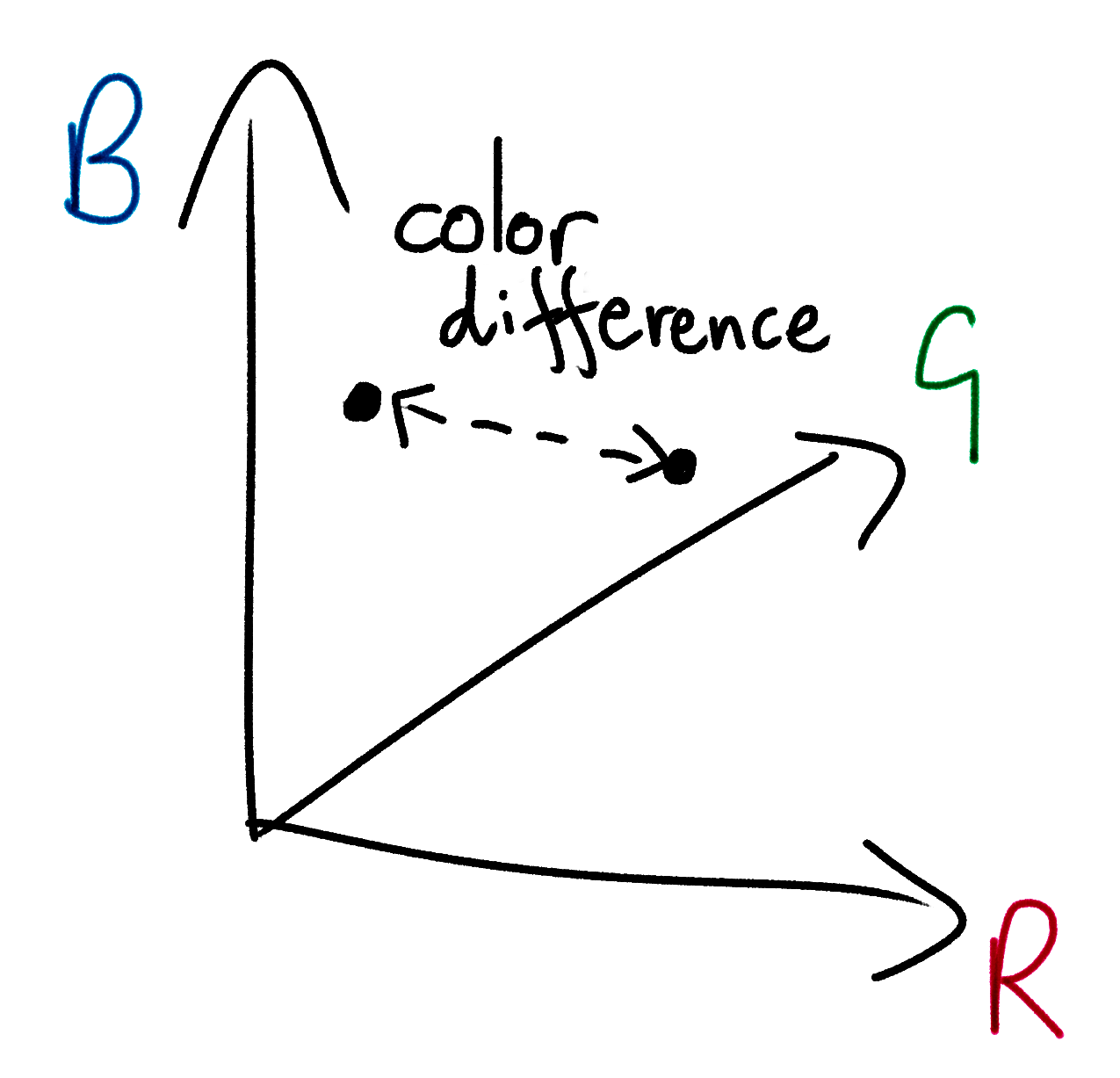
The Wikipedia page for “Color Difference” has some alternative, more complex ways to measure color similarity that account for the nuances of human perception. But humble, ancient Pythagoras does an excellent job.
For each square of your input image, use Pythagoras to find the source image that is nearest in RGB color space. Print out the names of your chosen images to the terminal.
4. Build the output image
Finally, paste together all the source images that you selected in the previous step onto an output image. Place each image in the position of the input image square that it is representing. Save it. You’re finished!
You’ll need to scale the source images down to avoid making the output image too large. Try, however, to keep the output image’s resolution high enough that you can still zoom in and see some of the details of the individual source images.
5. Pause and congratulate
You now have a program that creates photomosaics. Congratulations! Experiment with different images and different settings. Try changing the size of the squares that we divide our input image into. Try and hook your program up to your webcam so that you can produce photomosaics on-demand. Get ahead of the game and make your Christmas presents for next year.
Once you’ve done all of that, here are your 4 next steps:
- Attack the extensions below, where you’ll make your photomosaic program run much faster and produce output images with more fine-grained detail
- Tackle my other Programming Projects for Advanced Beginners - ASCII art, Game of Life and Tic-Tac-Toe AI
- Send me an email to let me know about your success. I’d love to know what you liked and didn’t like about the project, and any ideas you have for making the next one better
- Sign up for my newsletter at the bottom of this page to find out about new projects as they are published
Once again, congratulations!
NEW
Subscribe to my new "Programming Feedback for Advanced Beginners"
newsletter to receive concise weekly emails containing specific,
real-world ways to make your code cleaner and more professional.
Each week I review code sent to me by one of my readers. I highlight
the things that I like, discuss the
things that I think could be better, and offer suggestions for how
the author could make their code cleaner and easier to work with.
Subscribe now to receive these invaluable improvements in your inbox
every week, completely free.
Extensions
Extension 1. Speed up your program using caching
As you are by now aware, image processing can be quite slow. This is because it is a lot of work. Even a relatively low-resolution 1000x1000 image contains one million pixels, and iterating through all of them is exhausting. What’s more, we are doing a lot of calculation in our own, unoptimized code. We are not pushing much work off to our image processing library, which probably contains many low-level niceties that speed up operations on large collections of pixels. In general, the more work you can get your image processing library to do for you, the faster your program will be.
However, we can still gain a huge amount of speedup by tuning our own code. Let’s start by measuring how long each step of our program takes to find out where the bottlenecks are. Add some print statements to display some rough timing information:
start_time = Time.now
do_some_stuff()
end_time = Time.now
duration = end_time - start_time

print("Doing some stuff took: " + duration + " seconds")
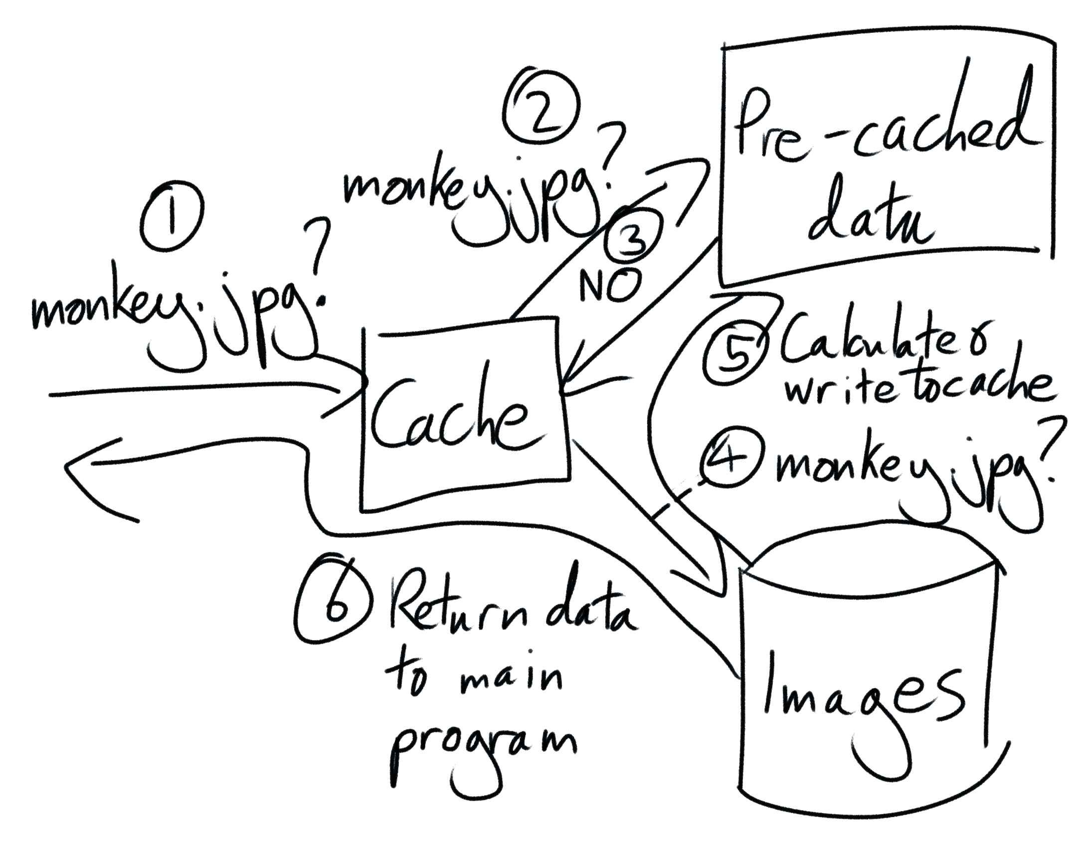
Once you’ve added this logging, you may notice that one of the slowest steps in your program is calculating the average colors of your source images. This step will be our first target for optimization.
We’ll attack it using a technique called caching. Caching means saving the result of a calculation so that you can re-use it again later, without having to re-do all of the work that went into producing it. We’ll use caching to take advantage of the facts that you probably don’t change your source images very often, and that if your source images don’t change, the results of your average color calculations don’t change either.
Right now the problem is that, once our program finishes, all of our precious variables disintegrate. They take all of our average color data with them, like so much sugar in so much coffee in a black hole. Let’s save our data from the abyss by writing it to something more persistent, like a file on your hard drive. Then the next time our program runs we’ll tell it to reload the data from this file, instead of having to calculate it all again.
Update our program so that, once we have calculated all of the average colors of our source images, we write the results to a file in a structured format like JSON (if you haven’t come across JSON before then don’t worry, Google has). This file will be our cache.
# In the file `mean_rgb_cache.json`:

{
  # FILENAME => AVERAGE COLOR
  # ...
  "family_lunch.jpg" => (135, 96, 42),
  "before_the_explosion.jpg" => (142, 99, 39),
  "what_was_i_thinking.jpg" => (140, 103, 49),
  "keep_for_blackmail.jpg" => (144, 101, 52),
  # ...
}
Now that we’ve created our cache, update our program again so that it loads it. Before calculating the average color of our source images, first check whether a cache file exists. If a file does exist, instead skip re-calculation, load it, and parse its cached data. Since loading a small data file is a much faster operation than loading and processing hundreds of images, this will speed up our program significantly.
Caching is a powerful technique, but it’s comes with plenty of gotchas. Caching will not speed up the first run of your program, since if no cache file exists then you still need to do all of the computation from scratch. In addition, if your source images do change, your cache file will become invalid and stale! Data for new images will be missing and, even more perniciously, data for updated images will be incorrect.
To prevent our cache from becoming stale, you need to manually “bust” the cache whenever our source images change. The most straightforward but naive way to do this is to simply delete the cache file. This will prevent your program from loading any out-of-date data, but at the cost of forcing it to re-run all of the average color calculations from scratch, even for old source images that didn’t change.
Happily, this cost can be minimized. We can have our cake, eat it, and cache the recipe so that we can make as many additional cakes as we want. To do this, load the cache file at the start of our program, as normal. Then, when our program wants to know the average color of a source image, it will ask our cache. If our cache already has a pre-calculated result available, it will instantly return it it. If it doesn’t, it will fetch the image, calculate its average color, and return the result. Crucially, it should also write this result to the cache so that it remembers it the next time we ask it for this image’s average color. This allows us to add new images to our cache on the fly, without having to delete all of our existing data.
Solving the problem of existing images that change underneath us is harder, but it can be done by using “hashing” and carefully chosen “cache keys”. Extension to the extension - use Google to work out how to make your cache deal with images that are updated, without their filename changing.
Caching is a very common technique - think about how you could apply it to other projects you have worked on. However, don’t try to optimize programs that don’t need optimizing! Caching can speed up your code, but it also makes it more complex. Whether that’s a worthwhile tradeoff depends on your situation. If a program is already fast enough (whatever that means for you), don’t worry about making it faster.
Extension 2. Speed up your program using pre-computation
With the average color of each source image cached and calculated, all that remains is to match source images to input squares, This is tractable enough when you have 1,000 or so source images, but what if you had 1,000,000? Or 10,000,000? Each comparison between a source image and an input square is very quick, but even something very quick can add up to something very slow if you do it enough times.
One way to solve this problem is with an index. An index is a way of structuring data that makes it faster to search through. Indexes are most commonly used in databases, and they’re how Twitter is able to so quickly retrieve the profile and tweets of @RobJHeaton without sequentially searching through the data of all of its users and bots.
Our index data structure will be a map from RGB colors to lists (or buckets) of source images with similar (but not necessarily identical) average colors. Then, when we want to select a source image for an input square, we only need to compare our input square to the source images in the nearest bucket in RGB space. This will be much, much faster than looking at every single image.
# We store our index in a data structure like:

{
  # ...
  (140, 100, 40) => [
    "family_lunch.jpg",
    "before_the_explosion.jpg"
  ],
  (140, 100, 50) => [
    "what_was_i_thinking.jpg",
    "keep_for_blackmail.jpg"
  ],
  # ...
}
To generate our index, we’ll take each source image’s average color and round the R, G, and B values to the nearest (for example) 10.
(151, 242, 9) ======> (150, 240, 10)
(1, 252, 45) ======> (0, 250, 50)
We’ll build a map (or hash, or dictionary, or whatever your language calls it) that maps from rounded RGB values to arrays of source images. Now when we come to choose a source image for an input square, we’ll round the input square’s RGB average color to the nearest 10, in the same way as we did for source images. We’ll use our map to get an array of the source images whose average colors also round to this value. We can then either iterate through each image in the bucket to find the closest one, or choose from them randomly since we know that their all at least decent matches.
For example, suppose an input square’s average color is (144, 99, 39). This rounds to (140, 100, 40). We look in our index (see above) and immediately find that the closest source images are family_lunch.jpg and before_the_explosion.jpg. We choose an image from these 2 options.
If the the index does not contain any source images for the input square’s RGB value, then we’ll have to look at some other nearby RGB values. Or we could just throw in a totally random source image and call it art.
Once you’ve implemented this optimization, make sure that you really understand it and can to articulate why this approach is generally faster. Why are we doing less work? Are there any edge-case situations that it might not be faster for?
Extension to the extension - read about database indexes, and try to understand how they are roughly related to what we have done here.
Further extension to the extension - we can combine this optimization with our previous one and cache our buckets! If we write our buckets to a file as JSON then we won’t have to recalculate them every time we run our program. Do this. Look at the rest of our program. Is there anywhere else where we are repeating work that we don’t have to?
Extension 3. Fine detail
We are selecting source images for input squares by comparing their overall average colors. This is very effective, but we can do even better. With just a few adjustments we can send our photomosaic to art school, and teach it how to capture fine detail.
We’ll do this by dividing our source images and input squares into four quarters, and separately calculating the average color of each quarter. Then, when calculating the distance between two images, we’ll calculate and combine the distance between all four pairs of quarters individually. This will teach our program to choose source images that better reflect the sub-structure of each input square.
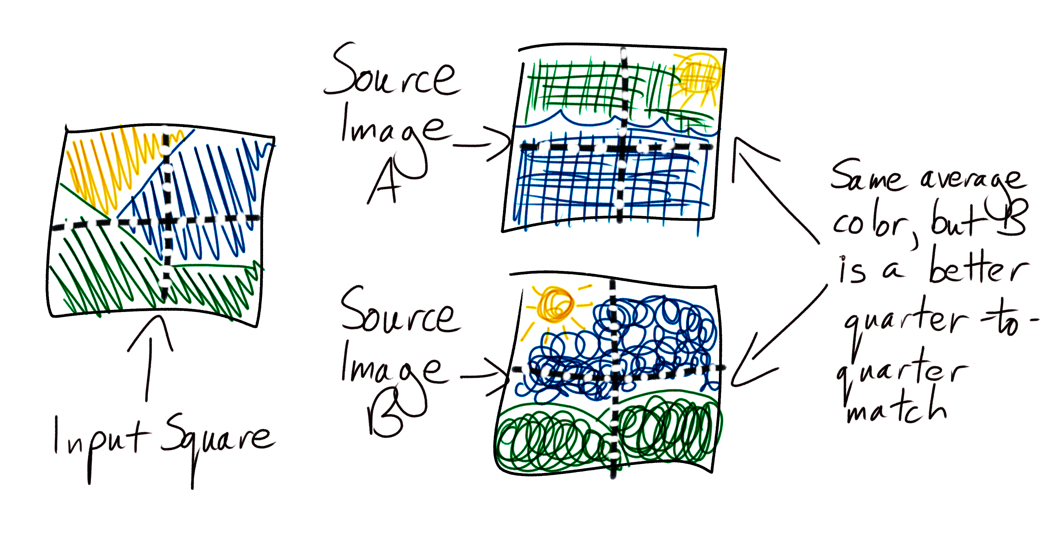
Now instead of one distance between a pair of images, we have four. Before we can compare different source images and choose the one that most closely matches an input square, we need to combine these four numbers into one. We can do this in many different ways, each of which will produce subtly different mosaics. Start by calculating their mean, then investigate using the median, harmonic mean, and any other distance metrics you can find on the internet. See which ones produce the best results.
Adapt our cache to work with our new fine-detail code. Try increasing the number of segments in each image to get even more precision. Try adapting this approach to whole images, and compare images in your albums to find those with similar color structures.
This is a programming project for Advanced Beginners. If you’ve completed all the introductory programming tutorials you can find and want to sharpen your skills on something bigger, this project is for you. You’ll get thrown in at the deep end. But you’ll also get gentle reminders on how to swim, as well as some new tips on swimming best practices. You can do it using any programming language you like, and if you get stuck I’ve written some example code that you can take inspiration from.
Subscribe to my new "Programming Feedback for Advanced Beginners" newsletter to receive concise weekly emails containing specific, real-world ways to make your code cleaner and more professional.
Each week I review code sent to me by one of my readers. I highlight the things that I like, discuss the things that I think could be better, and offer suggestions for how the author could make their code cleaner and easier to work with.
Subscribe now to receive these invaluable improvements in your inbox every week, completely free.
You may have come across photomosaics before - big pictures built out of thousands of other tiny pictures. In this project you’re going to build a photomosaic creator.
Unlike most other advanced beginner projects, a photomosaic creator is an extremely useful and practical tool. You can use it to mass-produce heartfelt, cheap, and easy presents for your friends and family. You can use it to create deep art with hidden meaning. You can make a picture of a delightful puppy out of thousands of pictures of murderous sharks, or a picture of a murderous shark out of thousands of pictures of delightful puppies. What do these works mean? Are they anti-capitalist, or pro? You don’t even have to decide.
The Plan
As in all Programming Projects for Advanced Beginners, we’ll build our program out of small components and intermediate milestones that we can test and verify individually. If small components and intermediate milestones are new concepts to you then you can either take a quick detour through my previous programming projects (here’s #1, #2 and #3), or push ahead with this project and pick things up as you go along.
We’ll start by sketching out a brief plan, and then get right on to coding. Before reading any further, spend a few minutes drawing up a plan of your own. What should we work on first? What about after that? What sub-problems will we need to solve? What intermediate milestones can we use to make sure we’re heading in the right direction? How can we test each milestone individually, even if we haven’t yet finished the entire program?
Take some time to think about the problem and devise your own plan before you continue - this is an important skill to develop.
My plan
Before I describe the plan that I came up with, let’s agree on some terminology to refer to the different pieces of our project. These aren’t official, technical definitions - they’re just names that I’ve made up for this project.
- Input image - the original image that we are going to recreate
- Output image - the finished photomosaic version of the input image
- Source images - the smaller images that the output image is made out of
We’ll also talk a lot about image processing libraries. An image processing library is a pre-written set of tools for loading and working with images. Almost every programming language has one (or several); have a look at section 1 of my ASCII art project for more advice on getting one set up.
For my plan I’ve come up with 7 steps:
1a. Use an image processing library to load an input image into your code. Paste your input image into a new output image. Mess around with it - rotate it, resize it, add a caption, and generally get familiar with your image processing library. 1b. Divide the input image into squares, and calculate the average color of each square 1c. A quick diversion - create an output image out of squares of these average colors. This will be a pixellated version of your input image! 2a. Find an initial set of 100 source images. Write a script that crops them all to squares and saves the cropped versions 2b. Calculate the average color of each source image
- For each section of the input image, find the source image with the closest average color
- Paste each of these source images into the output image in the appropriate location. You have a photomosaic!
Here’s a map of the system we’re aiming for:
We may change direction or get a little lost on the way, but at least we now have a solid idea of where we’re heading. I’ll race you there.
(note that this is not actually a race and you should take as much time as you need)
1a. Load the input image
Start by using your image processing library to load your input image. Make sure that the library is working correctly and start to get acquainted with its functionality and documentation. Experiment a bit. For example:
- Print the height and width of your image
- Shrink your image by 50%
- Rotate your image 180 degrees
- Draw a big red rectangle in the middle of your image
- Apply some Instagram-style filters
- Make an artistic collage of several different images
Express yourself. Think of this as finger-painting in code. There’s no right or wrong way to finger-paint.
1b. Divide and calculate
Next, divide your image up into squares, around 50x50 pixels in size, and for each square calculate the average color. Keep in mind that we’re going to reuse this code for calculating the average color of our source images too.
Image processing libraries load images as an array (or sometimes an “array of arrays”) of pixels. Each pixel is represented as an RGB tuple, a group of 3 numbers between 0 and 255 that represent the amount of red, green and blue in the pixel. Red, green and blue are the primary colors of light, and in the right proportions can be combined to create every single other color in existence.
The average color of an image section is simply the combination of the average red, green and blue values of its pixels. For example, if your pixels are:
[
(100, 71, 150),
(50, 71, 200),
(0, 71, 100),
]
then their average color is:
red = (100 + 50 + 0) / 3 = 50
green = (71 + 71 + 71) / 3 = 71
blue = (150 + 200 + 100) / 3 = 150
=> (50, 71, 150)
For more examples of working with pixels, arrays of arrays, and RGB values, see section 1 of my ASCII art project.
For now, don’t worry about doing anything with the average colors that you calculate - just print them to the terminal and make sure they look plausible. At the very least, are all the numbers between 0 and 255?
1c. Pixellate
This step isn’t part of the main project, but it is well worth a quick detour. Take the average colors that you just calculated and construct a new image out of squares of these average colors. This output image should look like a pixellated version of your input.
![]()
Experiment with changing the size of the squares. What effect does this have?
2a. Crop the source images
Now we’ll turn our attention to our source images. These are the small pictures that our larger output image will be built out of.
First, find an initial set of source images. A copy of the Photos directory on your computer is perfect. Alternatively Kaggle, a machine learning competition platform, has some good data sets of pictures of flowers, volcanoes and honey bees. Image processing is slow, so start with a small selection of 100 or so. We’ll add more once we’ve tuned our code’s performance.
Since we’re dividing our input image up into squares, we’ll need our source images to be squares too. Write a new script, separate from what you’ve written so far, that crops your source images down to squares. Trim each image to a square, where each side is the size of the original image’s shortest side. For example, if an image is 1200x800 pixels, crop it to 800x800. If it is 500x750, crop it to 500x500. Your script should save the cropped images in a new directory.
2b. Process the source images
Put the cropping script to one side and go back to your main program. In this program you’re already calculating the average color of each square of your input image. Use the same code to load and calculate the average color of each source image. Print the results out to the terminal.
3. Match source images to input squares
For each square in your input image, find the source image with the most similar average color. There are lots of different ways to do this; we’ll go with “Euclidean distance in RGB color space”. This is a ten-dollar way of saying:
This equation is Pythagoras’s Theorem in 3-dimensions. You may already be familiar with Pythagoras’s Theorem in 2-dimensions from maths lessons and everyday geometry. If you plotted your two colors as points on a set of 3-dimensional axes (one axis for each RGB value) this equation would give you the physical distance between the two points. This distance will be small for similar colors, and large for unrelated ones.
The Wikipedia page for “Color Difference” has some alternative, more complex ways to measure color similarity that account for the nuances of human perception. But humble, ancient Pythagoras does an excellent job.
For each square of your input image, use Pythagoras to find the source image that is nearest in RGB color space. Print out the names of your chosen images to the terminal.
4. Build the output image
Finally, paste together all the source images that you selected in the previous step onto an output image. Place each image in the position of the input image square that it is representing. Save it. You’re finished!
You’ll need to scale the source images down to avoid making the output image too large. Try, however, to keep the output image’s resolution high enough that you can still zoom in and see some of the details of the individual source images.
5. Pause and congratulate
You now have a program that creates photomosaics. Congratulations! Experiment with different images and different settings. Try changing the size of the squares that we divide our input image into. Try and hook your program up to your webcam so that you can produce photomosaics on-demand. Get ahead of the game and make your Christmas presents for next year.
Once you’ve done all of that, here are your 4 next steps:
- Attack the extensions below, where you’ll make your photomosaic program run much faster and produce output images with more fine-grained detail
- Tackle my other Programming Projects for Advanced Beginners - ASCII art, Game of Life and Tic-Tac-Toe AI
- Send me an email to let me know about your success. I’d love to know what you liked and didn’t like about the project, and any ideas you have for making the next one better
- Sign up for my newsletter at the bottom of this page to find out about new projects as they are published
Once again, congratulations!
Subscribe to my new "Programming Feedback for Advanced Beginners" newsletter to receive concise weekly emails containing specific, real-world ways to make your code cleaner and more professional.
Each week I review code sent to me by one of my readers. I highlight the things that I like, discuss the things that I think could be better, and offer suggestions for how the author could make their code cleaner and easier to work with.
Subscribe now to receive these invaluable improvements in your inbox every week, completely free.
Extensions
Extension 1. Speed up your program using caching
As you are by now aware, image processing can be quite slow. This is because it is a lot of work. Even a relatively low-resolution 1000x1000 image contains one million pixels, and iterating through all of them is exhausting. What’s more, we are doing a lot of calculation in our own, unoptimized code. We are not pushing much work off to our image processing library, which probably contains many low-level niceties that speed up operations on large collections of pixels. In general, the more work you can get your image processing library to do for you, the faster your program will be.
However, we can still gain a huge amount of speedup by tuning our own code. Let’s start by measuring how long each step of our program takes to find out where the bottlenecks are. Add some print statements to display some rough timing information:
start_time = Time.now
do_some_stuff()
end_time = Time.now
duration = end_time - start_time
print("Doing some stuff took: " + duration + " seconds")
Once you’ve added this logging, you may notice that one of the slowest steps in your program is calculating the average colors of your source images. This step will be our first target for optimization.
We’ll attack it using a technique called caching. Caching means saving the result of a calculation so that you can re-use it again later, without having to re-do all of the work that went into producing it. We’ll use caching to take advantage of the facts that you probably don’t change your source images very often, and that if your source images don’t change, the results of your average color calculations don’t change either.
Right now the problem is that, once our program finishes, all of our precious variables disintegrate. They take all of our average color data with them, like so much sugar in so much coffee in a black hole. Let’s save our data from the abyss by writing it to something more persistent, like a file on your hard drive. Then the next time our program runs we’ll tell it to reload the data from this file, instead of having to calculate it all again.
Update our program so that, once we have calculated all of the average colors of our source images, we write the results to a file in a structured format like JSON (if you haven’t come across JSON before then don’t worry, Google has). This file will be our cache.
# In the file `mean_rgb_cache.json`:
{
# FILENAME => AVERAGE COLOR
# ...
"family_lunch.jpg" => (135, 96, 42),
"before_the_explosion.jpg" => (142, 99, 39),
"what_was_i_thinking.jpg" => (140, 103, 49),
"keep_for_blackmail.jpg" => (144, 101, 52),
# ...
}
Now that we’ve created our cache, update our program again so that it loads it. Before calculating the average color of our source images, first check whether a cache file exists. If a file does exist, instead skip re-calculation, load it, and parse its cached data. Since loading a small data file is a much faster operation than loading and processing hundreds of images, this will speed up our program significantly.
Caching is a powerful technique, but it’s comes with plenty of gotchas. Caching will not speed up the first run of your program, since if no cache file exists then you still need to do all of the computation from scratch. In addition, if your source images do change, your cache file will become invalid and stale! Data for new images will be missing and, even more perniciously, data for updated images will be incorrect.
To prevent our cache from becoming stale, you need to manually “bust” the cache whenever our source images change. The most straightforward but naive way to do this is to simply delete the cache file. This will prevent your program from loading any out-of-date data, but at the cost of forcing it to re-run all of the average color calculations from scratch, even for old source images that didn’t change.
Happily, this cost can be minimized. We can have our cake, eat it, and cache the recipe so that we can make as many additional cakes as we want. To do this, load the cache file at the start of our program, as normal. Then, when our program wants to know the average color of a source image, it will ask our cache. If our cache already has a pre-calculated result available, it will instantly return it it. If it doesn’t, it will fetch the image, calculate its average color, and return the result. Crucially, it should also write this result to the cache so that it remembers it the next time we ask it for this image’s average color. This allows us to add new images to our cache on the fly, without having to delete all of our existing data.
Solving the problem of existing images that change underneath us is harder, but it can be done by using “hashing” and carefully chosen “cache keys”. Extension to the extension - use Google to work out how to make your cache deal with images that are updated, without their filename changing.
Caching is a very common technique - think about how you could apply it to other projects you have worked on. However, don’t try to optimize programs that don’t need optimizing! Caching can speed up your code, but it also makes it more complex. Whether that’s a worthwhile tradeoff depends on your situation. If a program is already fast enough (whatever that means for you), don’t worry about making it faster.
Extension 2. Speed up your program using pre-computation
With the average color of each source image cached and calculated, all that remains is to match source images to input squares, This is tractable enough when you have 1,000 or so source images, but what if you had 1,000,000? Or 10,000,000? Each comparison between a source image and an input square is very quick, but even something very quick can add up to something very slow if you do it enough times.
One way to solve this problem is with an index. An index is a way of structuring data that makes it faster to search through. Indexes are most commonly used in databases, and they’re how Twitter is able to so quickly retrieve the profile and tweets of @RobJHeaton without sequentially searching through the data of all of its users and bots.
Our index data structure will be a map from RGB colors to lists (or buckets) of source images with similar (but not necessarily identical) average colors. Then, when we want to select a source image for an input square, we only need to compare our input square to the source images in the nearest bucket in RGB space. This will be much, much faster than looking at every single image.
# We store our index in a data structure like:
{
# ...
(140, 100, 40) => [
"family_lunch.jpg",
"before_the_explosion.jpg"
],
(140, 100, 50) => [
"what_was_i_thinking.jpg",
"keep_for_blackmail.jpg"
],
# ...
}
To generate our index, we’ll take each source image’s average color and round the R, G, and B values to the nearest (for example) 10.
(151, 242, 9) ======> (150, 240, 10)
(1, 252, 45) ======> (0, 250, 50)
We’ll build a map (or hash, or dictionary, or whatever your language calls it) that maps from rounded RGB values to arrays of source images. Now when we come to choose a source image for an input square, we’ll round the input square’s RGB average color to the nearest 10, in the same way as we did for source images. We’ll use our map to get an array of the source images whose average colors also round to this value. We can then either iterate through each image in the bucket to find the closest one, or choose from them randomly since we know that their all at least decent matches.
For example, suppose an input square’s average color is (144, 99, 39). This rounds to (140, 100, 40). We look in our index (see above) and immediately find that the closest source images are family_lunch.jpg and before_the_explosion.jpg. We choose an image from these 2 options.
If the the index does not contain any source images for the input square’s RGB value, then we’ll have to look at some other nearby RGB values. Or we could just throw in a totally random source image and call it art.
Once you’ve implemented this optimization, make sure that you really understand it and can to articulate why this approach is generally faster. Why are we doing less work? Are there any edge-case situations that it might not be faster for?
Extension to the extension - read about database indexes, and try to understand how they are roughly related to what we have done here.
Further extension to the extension - we can combine this optimization with our previous one and cache our buckets! If we write our buckets to a file as JSON then we won’t have to recalculate them every time we run our program. Do this. Look at the rest of our program. Is there anywhere else where we are repeating work that we don’t have to?
Extension 3. Fine detail
We are selecting source images for input squares by comparing their overall average colors. This is very effective, but we can do even better. With just a few adjustments we can send our photomosaic to art school, and teach it how to capture fine detail.
We’ll do this by dividing our source images and input squares into four quarters, and separately calculating the average color of each quarter. Then, when calculating the distance between two images, we’ll calculate and combine the distance between all four pairs of quarters individually. This will teach our program to choose source images that better reflect the sub-structure of each input square.
Now instead of one distance between a pair of images, we have four. Before we can compare different source images and choose the one that most closely matches an input square, we need to combine these four numbers into one. We can do this in many different ways, each of which will produce subtly different mosaics. Start by calculating their mean, then investigate using the median, harmonic mean, and any other distance metrics you can find on the internet. See which ones produce the best results.
Adapt our cache to work with our new fine-detail code. Try increasing the number of segments in each image to get even more precision. Try adapting this approach to whole images, and compare images in your albums to find those with similar color structures.