PFAB #16: How to make your code faster and why you often shouldn't bother
14 Jun 2020
This post is part of my “Programming Feedback for Advanced Beginners” series, in which you make the leap from cobbling programs together to writing elegant, thoughtful code. Subscribe now to receive PFAB in your inbox, every fortnight, entirely free.
This week on Programming Feedback for Advanced Beginners we’re going to talk about speed. To do this we’re going to analyze some code that was sent to me by PFAB reader Justin Reppert. Justin’s code is a solution to Programming Projects for Advanced Beginners #1: ASCII art. Justin’s program works perfectly and his code is neat and tidy, but he still wants to know:
“How can I make it faster?”
Whenever I’m asked this question, my first response is always “why does it need to be faster?” Fast code is of course better than slow code, all else being equal. But you should always ask yourself whether the execution speed of your particular program actually matters. Is it fast enough already? If it was a bit faster, would the world be an appreciably better place? Writing faster code takes time that could be profitably spent elsewhere, and optimized code is often more complex and more bug-prone than its dawdling brethren. Unless my code’s speed is actively costing me money or happiness, I’d almost always rather spend my energy on making it more reliable or readable than on making it faster. Justin should be proud of his code just the way it is.
To his credit, Justin recognizes that the speed of his ASCII art generation program is not important. He can afford to wait a few seconds for his command line masterpieces, and he understands that great art takes time. Nonetheless, optimizing his code’s performance is still an interesting educational exercise. So, with all the above caveats in mind, here’s how I would do it.
What does Justin’s program do?
Before we look at how to speed up Justin’s program, let’s talk about how it works. Justin’s program takes in an input image file in JPG format. It analyzes the image and prints it to the user’s terminal using colorful ASCII characters. Here’s the code.
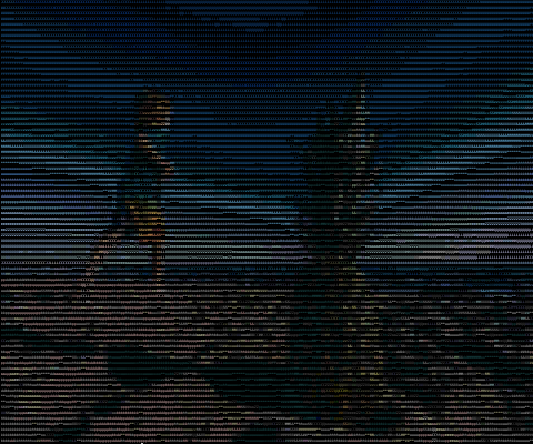
Justin wants to speed up the part of his program responsible for choosing the colors that are printed to the terminal. In an image file, the color of a pixel is stored as 3 numbers that describe the amount of Red, Green, and Blue in the pixel respectively. Each of these numbers is an integer between 0 and 255; for example, the shade of blue in the Facebook logo is represented as (59,89,152). This trio of numbers is called a color’s RGB value. This means that each pixel in an image file can be any of 256 * 256 * 256 =~ 16MM possible colors.
However, using a terminal as a canvas imposes restrictions on an artist. Characters can only be printed to a terminal using a limited subset of these 16MM possible colors. The ANSI extended standard defines 255 colors that compliant terminals should be capable of displaying. This means that in order to display an image in a terminal, we need to round the color of each pixel in our file to the closest ANSI color. Justin’s sensible, straightforward method of doing this is to, for each pixel:
- Calculate the distances between the pixel color and each ANSI color using 3-D Pythagoras’s Theorem
- Return the ANSI color closest to the pixel color
This is a practical and logical algorithm. However, Justin tells me that he feels uneasy about the amount of computational work it requires. His algorithm has to calculate the distance between every pixel color and every terminal color. Even for a scaled down image of 80x80 pixels, this is 80 * 80 * 256 =~ 1.6MM separate distances for a single image. Justin’s program is perfectly speedy and completes in a few seconds, but he wonders whether much of the work it does could be avoided.
It could.
How can we speed up choosing colors?
I can think of several ways we can speed up Justin’s program:
- Use a faster algorithm for finding the closest terminal color to a given pixel color
- Use the same algorithm, but use a cache to reuse past work where possible instead of starting fresh for each image pixel
- Use the same algorithm, but precompute some amount of data before starting
This week we’ll look into option 1: use a faster algorithm. We’ll look into options 2 and 3 in the next edition of PFAB.
1. Use a faster algorithm
Using a faster algorithm is the simplest and most effective way of speeding up Justin’s code. If your algorithm isn’t fast enough, it makes sense to look for a faster one. But despite being the best approach, I think that it’s also the most boring. Designing a faster color-matching algorithm will teach you a couple of tricks and ways of thinking that might indirectly come in useful once or twice in your life. However, it won’t give you any generally-applicable lessons for structuring your future programs and systems. Nonetheless, this week we’ll discuss it, see how to do it, then pretend it never happened and look at the more exciting - if less immediately practical - options next time.
Note that even the zippy algorithm I’m about to describe is almost certainly not the absolute fastest method out there. Despite this, it still gives us a good 30x speedup over Justin’s current approach. You can always make even a somewhat optimized piece of code faster. If we really needed to make the program as fast as physically possible - cost and complexity be damned - then we would write it in C or hand-create the assembly code. Computer scientist Donald Knuth is famous for saying that “premature optimization is the root of all evil”. That would make us the Satan of speed.
Fortunately we don’t have to do anything too villainous in order to pick up a good chunk of extra velocity. We can exploit the fact that the ANSI terminal colors are spaced regularly around RGB color space. Each RGB value is always one of [0, 95, 135, 175, 215, 255] (apart from a few exceptions that we’ll talk about later). Even though this list shows us that ANSI colors aren’t spaced evenly, their RGB values still form a rectangular (or cuboid, in 3-D) grid. This is all we need.
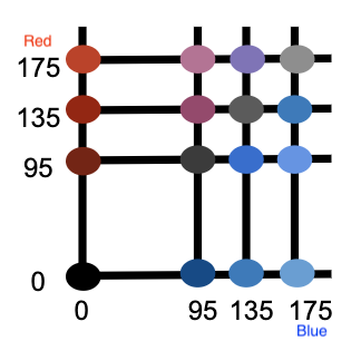
Suppose that we’re trying to find the best matching terminal color for a pixel. Since we know the values at which the effective ANSI gridlines are drawn, we don’t actually have to compare our pixel color to every possible terminal color (which is what Justin currently does). Instead, we can look at the list of values at which gridlines are drawn, and snap each of our pixel’s R, G, and B values to the nearest of these gridlines. Doing this for R, G, and B will give us a new, rounded RGB co-ordinate. Because ANSI terminal colors are arranged regularly, we know that there will be an ANSI color at this rounded co-ordinate. And if you think about it hard enough, we also know that this ANSI color will be the closest one to our original pixel color.
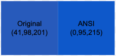
For example, suppose that we want to find the closest ANSI color to the pixel color (41, 98, 201). We remember that the RGB values of (most) ANSI colors are always [0, 95, 135, 175, 215, 255]. We snap our R, G, and B values to the nearest value in this list, giving us (0, 95, 215). We look this up and see that it indeed corresponds to a valid ANSI color. This is a much quicker calculation than performing 3-D Pythagoras’s Theorem 255 times.
Astute readers might notice that the full list of extended ANSI colors includes extra grayscale colors (white, black, and several shades of grey) at additional gridline values not used by non-gray colors.
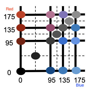
There are several ways we can adapt our algorithm to include these additional tones. For example, we could use the above process to snap our pixel RGB values to the nearest grayscale gridlines. If there is a valid ANSI color at this snapped point, we return it. If not, we return the ANSI color calculated in the previous paragraph. We’ve had enough fun for one day already, so a detailed analysis of this minor point is left to the reader.
Writing the faster code
I’ve updated Justin’s code to use this faster algorithm. You can read my new version here, or look at just the diff between our versions here. On my computer Justin’s original code takes a respectable 6.2s to process the sample image from his repo, but the updated algorithm zips through it in a mere 0.18s.
To find the closest gridline value to an R, G or B value, I found the gridline value with the minimum absolute difference between the gridline value and the original value. The absolute difference between two numbers is the difference between them, expressed as a positive number. The absolute difference between 5 and 8 is 3. The absolute difference between 10 and 1 is 9. In Python the absolute difference between two numbers x and y can be calculated by abs(x - y). This gave me the following code:
def rgb_to_ansi(rgb):
    # `snap_value` snaps an R, G, or B value to the
    # closest gridline value.
    def snap_value(val):
        return min(GRIDLINES, key=lambda el: abs(val - el))

    ansi_rgb = [snap_value(v) for v in rgb]
    # Map the snapped RGB value to an ANSI color code
    # (not important for an understanding of the
    # algorithm).
    return inverted_color_dict[str(ansi_rgb)]
Even this approach can be sped up. When snapping an RGB value to the nearest gridline, the code iterates through every value in GRIDLINES, even in situations where we intuitively know that we’ve already found the closest gridline. To save some work we could iterate through GRIDLINES in ascending order and return early once the absolute difference starts to increase. Once the absolute difference starts to increase, the fact that we’re iterating through the gridline values in ascending order means that we know we’ve found the closest value. We don’t need to calculate abs(val - g) for any further gridlines and can instead immediately return the closest value that we’ve found so far.
Suppose that we want to snap the number 120 to the closest gridline. Our calculations might look like this:
// We calculate abs(gridline - value) for each gridline
// value in ascending order:
GRIDLINES = [0, 95, 135, 175, 215, 255]

abs(120 - 0) = 120
abs(120 - 95) = 25
// The absolute difference is decreasing, so we keep
// going.

abs(120 - 135) = 15
// The absolute difference is still decreasing, so we
// still keep going.

abs(120 - 175) = 55
// The absolute difference has started to increase,
// so we immediately return the previous gridline
// value: 135.
I’m not entirely certain that this approach really is any quicker than simply using min. I think it probably is, but I’d need to time and compare them carefully in order to be sure. Even if this approach is quicker, in my opinion the increased complexity of the resulting code is unlikely to be worth the fractions of a second that you’ll save. Unless for your specific situation it is.
Conclusion
You can almost always speed up a piece of code, but speed doesn’t come for free. To quote myself from a few paragraphs ago: “Writing faster code takes time that could be profitably spent elsewhere, and optimized code is often more complex and more bug-prone than its dawdling brethren.” Sometimes these tradeoffs will be worth it, but often they won’t. Don’t feel bad about writing straightforward, moderately-paced code.
Create your own lo-fi art and implement the algorithm in this post yourself by tackling Programming Projects for Advanced Beginners #1: ASCII art.
Missed previous PFABs? Catch up with the full archives and learn how to make your programs shorter, clearer, and easier for other people to work with.
This post is part of my “Programming Feedback for Advanced Beginners” series, in which you make the leap from cobbling programs together to writing elegant, thoughtful code. Subscribe now to receive PFAB in your inbox, every fortnight, entirely free.
This week on Programming Feedback for Advanced Beginners we’re going to talk about speed. To do this we’re going to analyze some code that was sent to me by PFAB reader Justin Reppert. Justin’s code is a solution to Programming Projects for Advanced Beginners #1: ASCII art. Justin’s program works perfectly and his code is neat and tidy, but he still wants to know:
“How can I make it faster?”
Whenever I’m asked this question, my first response is always “why does it need to be faster?” Fast code is of course better than slow code, all else being equal. But you should always ask yourself whether the execution speed of your particular program actually matters. Is it fast enough already? If it was a bit faster, would the world be an appreciably better place? Writing faster code takes time that could be profitably spent elsewhere, and optimized code is often more complex and more bug-prone than its dawdling brethren. Unless my code’s speed is actively costing me money or happiness, I’d almost always rather spend my energy on making it more reliable or readable than on making it faster. Justin should be proud of his code just the way it is.
To his credit, Justin recognizes that the speed of his ASCII art generation program is not important. He can afford to wait a few seconds for his command line masterpieces, and he understands that great art takes time. Nonetheless, optimizing his code’s performance is still an interesting educational exercise. So, with all the above caveats in mind, here’s how I would do it.
What does Justin’s program do?
Before we look at how to speed up Justin’s program, let’s talk about how it works. Justin’s program takes in an input image file in JPG format. It analyzes the image and prints it to the user’s terminal using colorful ASCII characters. Here’s the code.
Justin wants to speed up the part of his program responsible for choosing the colors that are printed to the terminal. In an image file, the color of a pixel is stored as 3 numbers that describe the amount of Red, Green, and Blue in the pixel respectively. Each of these numbers is an integer between 0 and 255; for example, the shade of blue in the Facebook logo is represented as (59,89,152). This trio of numbers is called a color’s RGB value. This means that each pixel in an image file can be any of 256 * 256 * 256 =~ 16MM possible colors.
However, using a terminal as a canvas imposes restrictions on an artist. Characters can only be printed to a terminal using a limited subset of these 16MM possible colors. The ANSI extended standard defines 255 colors that compliant terminals should be capable of displaying. This means that in order to display an image in a terminal, we need to round the color of each pixel in our file to the closest ANSI color. Justin’s sensible, straightforward method of doing this is to, for each pixel:
- Calculate the distances between the pixel color and each ANSI color using 3-D Pythagoras’s Theorem
- Return the ANSI color closest to the pixel color
This is a practical and logical algorithm. However, Justin tells me that he feels uneasy about the amount of computational work it requires. His algorithm has to calculate the distance between every pixel color and every terminal color. Even for a scaled down image of 80x80 pixels, this is 80 * 80 * 256 =~ 1.6MM separate distances for a single image. Justin’s program is perfectly speedy and completes in a few seconds, but he wonders whether much of the work it does could be avoided.
It could.
How can we speed up choosing colors?
I can think of several ways we can speed up Justin’s program:
- Use a faster algorithm for finding the closest terminal color to a given pixel color
- Use the same algorithm, but use a cache to reuse past work where possible instead of starting fresh for each image pixel
- Use the same algorithm, but precompute some amount of data before starting
This week we’ll look into option 1: use a faster algorithm. We’ll look into options 2 and 3 in the next edition of PFAB.
1. Use a faster algorithm
Using a faster algorithm is the simplest and most effective way of speeding up Justin’s code. If your algorithm isn’t fast enough, it makes sense to look for a faster one. But despite being the best approach, I think that it’s also the most boring. Designing a faster color-matching algorithm will teach you a couple of tricks and ways of thinking that might indirectly come in useful once or twice in your life. However, it won’t give you any generally-applicable lessons for structuring your future programs and systems. Nonetheless, this week we’ll discuss it, see how to do it, then pretend it never happened and look at the more exciting - if less immediately practical - options next time.
Note that even the zippy algorithm I’m about to describe is almost certainly not the absolute fastest method out there. Despite this, it still gives us a good 30x speedup over Justin’s current approach. You can always make even a somewhat optimized piece of code faster. If we really needed to make the program as fast as physically possible - cost and complexity be damned - then we would write it in C or hand-create the assembly code. Computer scientist Donald Knuth is famous for saying that “premature optimization is the root of all evil”. That would make us the Satan of speed.
Fortunately we don’t have to do anything too villainous in order to pick up a good chunk of extra velocity. We can exploit the fact that the ANSI terminal colors are spaced regularly around RGB color space. Each RGB value is always one of [0, 95, 135, 175, 215, 255] (apart from a few exceptions that we’ll talk about later). Even though this list shows us that ANSI colors aren’t spaced evenly, their RGB values still form a rectangular (or cuboid, in 3-D) grid. This is all we need.
Suppose that we’re trying to find the best matching terminal color for a pixel. Since we know the values at which the effective ANSI gridlines are drawn, we don’t actually have to compare our pixel color to every possible terminal color (which is what Justin currently does). Instead, we can look at the list of values at which gridlines are drawn, and snap each of our pixel’s R, G, and B values to the nearest of these gridlines. Doing this for R, G, and B will give us a new, rounded RGB co-ordinate. Because ANSI terminal colors are arranged regularly, we know that there will be an ANSI color at this rounded co-ordinate. And if you think about it hard enough, we also know that this ANSI color will be the closest one to our original pixel color.
For example, suppose that we want to find the closest ANSI color to the pixel color (41, 98, 201). We remember that the RGB values of (most) ANSI colors are always [0, 95, 135, 175, 215, 255]. We snap our R, G, and B values to the nearest value in this list, giving us (0, 95, 215). We look this up and see that it indeed corresponds to a valid ANSI color. This is a much quicker calculation than performing 3-D Pythagoras’s Theorem 255 times.
Astute readers might notice that the full list of extended ANSI colors includes extra grayscale colors (white, black, and several shades of grey) at additional gridline values not used by non-gray colors.
There are several ways we can adapt our algorithm to include these additional tones. For example, we could use the above process to snap our pixel RGB values to the nearest grayscale gridlines. If there is a valid ANSI color at this snapped point, we return it. If not, we return the ANSI color calculated in the previous paragraph. We’ve had enough fun for one day already, so a detailed analysis of this minor point is left to the reader.
Writing the faster code
I’ve updated Justin’s code to use this faster algorithm. You can read my new version here, or look at just the diff between our versions here. On my computer Justin’s original code takes a respectable 6.2s to process the sample image from his repo, but the updated algorithm zips through it in a mere 0.18s.
To find the closest gridline value to an R, G or B value, I found the gridline value with the minimum absolute difference between the gridline value and the original value. The absolute difference between two numbers is the difference between them, expressed as a positive number. The absolute difference between 5 and 8 is 3. The absolute difference between 10 and 1 is 9. In Python the absolute difference between two numbers x and y can be calculated by abs(x - y). This gave me the following code:
def rgb_to_ansi(rgb):
# `snap_value` snaps an R, G, or B value to the
# closest gridline value.
def snap_value(val):
return min(GRIDLINES, key=lambda el: abs(val - el))
ansi_rgb = [snap_value(v) for v in rgb]
# Map the snapped RGB value to an ANSI color code
# (not important for an understanding of the
# algorithm).
return inverted_color_dict[str(ansi_rgb)]
Even this approach can be sped up. When snapping an RGB value to the nearest gridline, the code iterates through every value in GRIDLINES, even in situations where we intuitively know that we’ve already found the closest gridline. To save some work we could iterate through GRIDLINES in ascending order and return early once the absolute difference starts to increase. Once the absolute difference starts to increase, the fact that we’re iterating through the gridline values in ascending order means that we know we’ve found the closest value. We don’t need to calculate abs(val - g) for any further gridlines and can instead immediately return the closest value that we’ve found so far.
Suppose that we want to snap the number 120 to the closest gridline. Our calculations might look like this:
// We calculate abs(gridline - value) for each gridline
// value in ascending order:
GRIDLINES = [0, 95, 135, 175, 215, 255]
abs(120 - 0) = 120
abs(120 - 95) = 25
// The absolute difference is decreasing, so we keep
// going.
abs(120 - 135) = 15
// The absolute difference is still decreasing, so we
// still keep going.
abs(120 - 175) = 55
// The absolute difference has started to increase,
// so we immediately return the previous gridline
// value: 135.
I’m not entirely certain that this approach really is any quicker than simply using min. I think it probably is, but I’d need to time and compare them carefully in order to be sure. Even if this approach is quicker, in my opinion the increased complexity of the resulting code is unlikely to be worth the fractions of a second that you’ll save. Unless for your specific situation it is.
Conclusion
You can almost always speed up a piece of code, but speed doesn’t come for free. To quote myself from a few paragraphs ago: “Writing faster code takes time that could be profitably spent elsewhere, and optimized code is often more complex and more bug-prone than its dawdling brethren.” Sometimes these tradeoffs will be worth it, but often they won’t. Don’t feel bad about writing straightforward, moderately-paced code.
Create your own lo-fi art and implement the algorithm in this post yourself by tackling Programming Projects for Advanced Beginners #1: ASCII art.
Missed previous PFABs? Catch up with the full archives and learn how to make your programs shorter, clearer, and easier for other people to work with.