Three men were accused of selling firearms to South London gangs. At their 2012 trial in Croydon Crown Court, the prosecution played the jury a recording, taken undercover, of the trio allegedly arranging a sale. But the men’s lawyers claimed that the recording was a fake, and that the police had fabricated it by splicing together clips taken at different times. To prove that the evidence really was authentic, the Metropolitan Police turned to a technique called electrical network frequency (ENF) matching.
ENF matching exploits patterns in the frequency of the “mains hum” - the faint background noise emitted by an electrical grid as it pipes electricity around in order to power our homes and workplaces. The hum seeps into microphones and recordings, which is a pain for sound engineers, but surprisingly useful for forensic analysts.
To substantiate the recording, Dr Alan Cooper, an analyst on the Met, extracted the sound of its mains hum. He matched fluctuations in the hum’s frequency to frequency readings taken directly from the National Grid at the time of the alleged deal. Their close correspondence suggested that the recording had indeed been taken at the time that the prosecution claimed. He also used the hum’s continuity to show that it was indeed a single, undoctored clip. His analysis stuck, and the three men were convicted. Hume Bent was jailed for 17 years; Christopher McKenzie for 12. In a 2012 article, Cooper was quoted as saying that “[ENF analysis] is now starting to be used widely by [the Met], as well as [other police forces] around the world.”
ENF matching answers the question “here’s a recording, when was it was (probably) taken?” It’s a lively field of academic research but little has been written about it outside of paywalled papers, so in this post I’m going to describe the technical details for the interested layperson. I’ve also put up a readable, well-commented example implementation on Github.
Let’s begin.
Where does the mains hum come from?
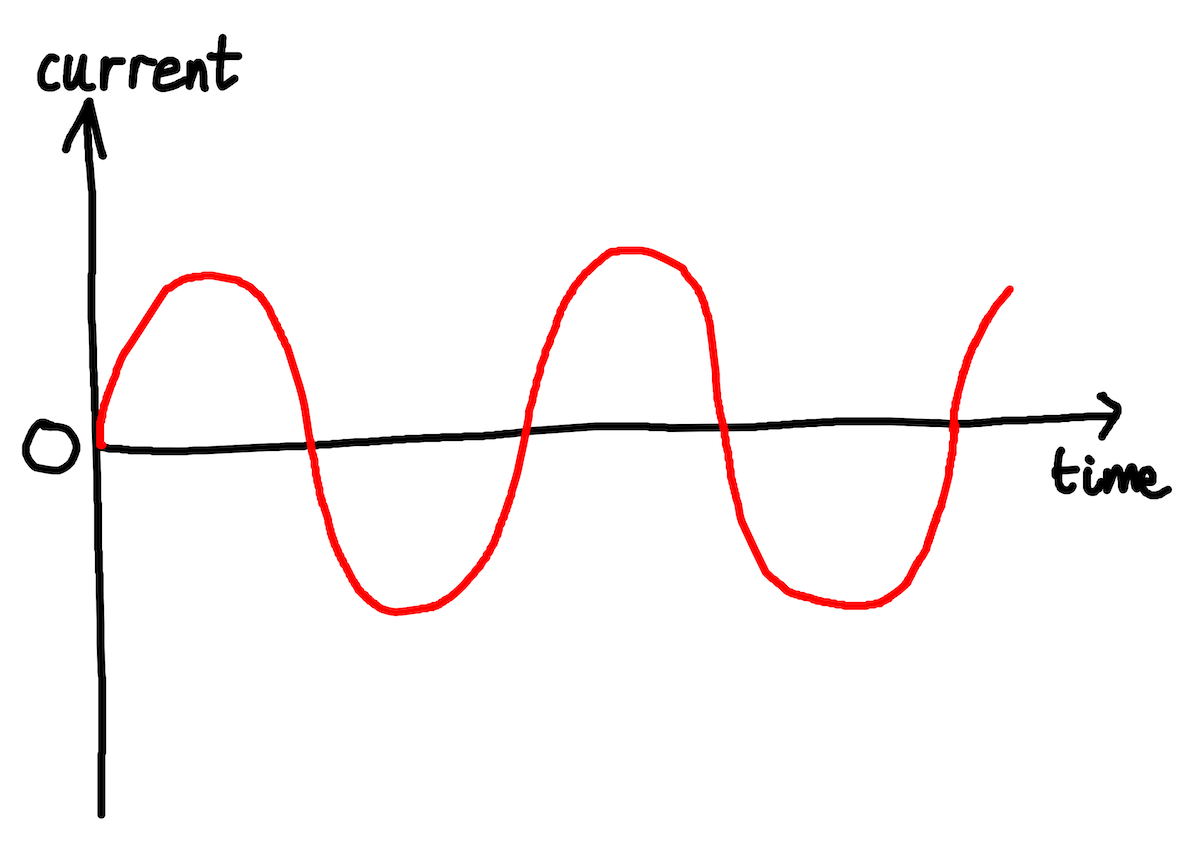
Power is transmitted through an electrical grid as alternating current (AC). This means that the current flowing through the grid’s cables constantly changes direction. In most regions - including Great Britain, where I live - the current’s direction switches 50 times a second, or 50Hz. In some other regions, like the US and Canada, it switches 60 times a second, or 60Hz. For the rest of this post we’ll talk from the point of view of Britain and other 50Hz grids.
Fig: Alternating current going backwards and forwards
This electrical back-and-forth causes some of the components that the current passes through to vibrate, very slightly, at the same frequency as the AC oscillation. This vibration causes a barely audible sound, also at 50Hz. This sound is the mains hum.
The British grid targets an electrical network frequency (ENF) of 50Hz. But in practice the frequency varies slightly and randomly around this target, as power demand fluctuates (49.8Hz-50.2Hz is a normal range). The grid is a single, connected system, so when ENF wanders, it wanders in synchrony across the whole of Great Britain (Northern Ireland uses a separate grid that it shares with the Republic of Ireland). The ENF in Glasgow is always exactly the same as in London, Bristol, and Swansea.
Different countries have different grid configurations. Many, like Nordic Europe, share a grid with their neighbours. A few, like Japan, have multiple grids. Regardless of a grid’s size, the current flowing through it oscillates in perfect synchrony, at exactly the same frequency, throughout the whole grid.
Fig: electrical grids of Europe and North Africa. Source: Wikipedia, licensed under CC BY-SA 3.0
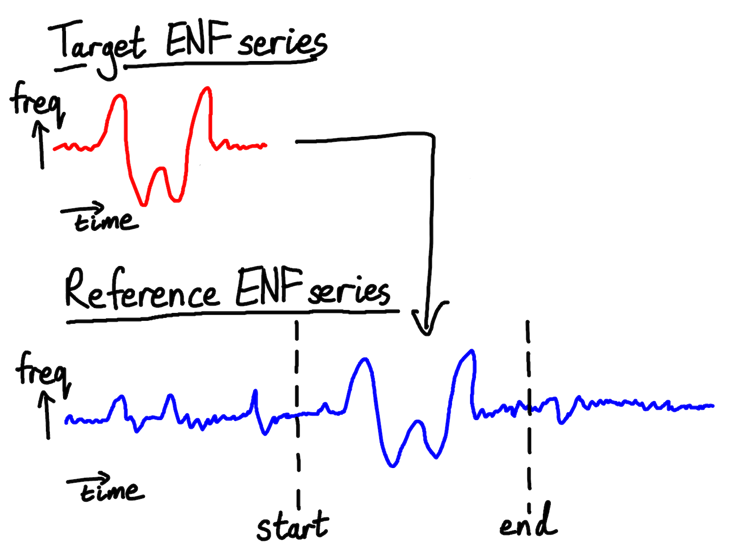
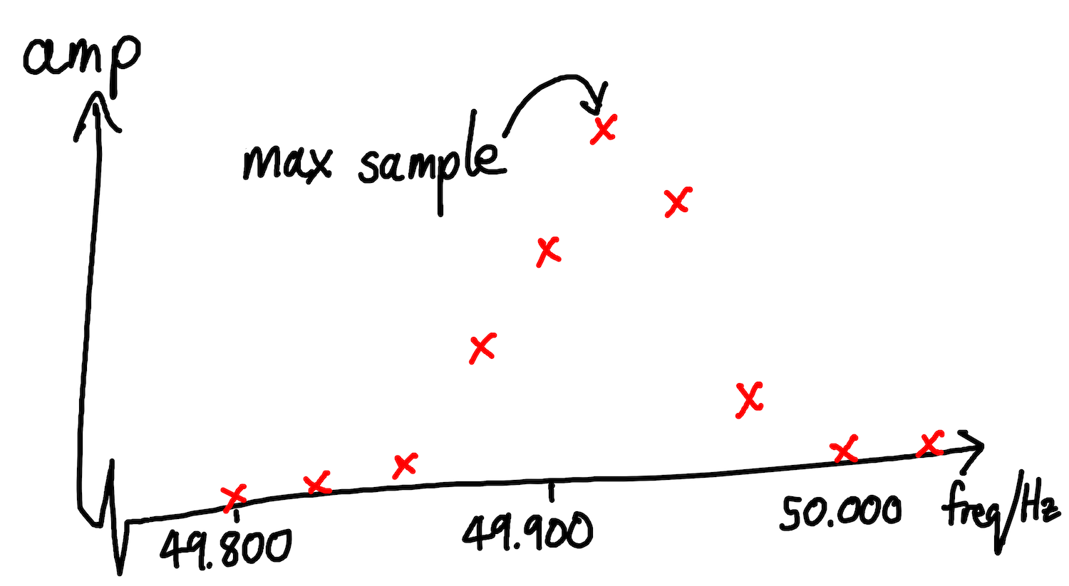
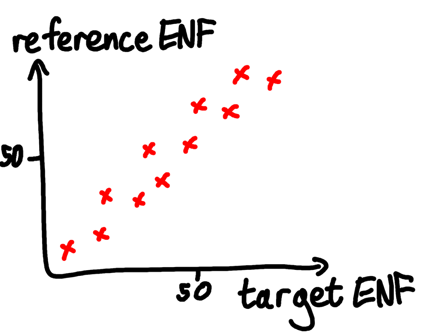
When the mains hum produced by AC oscillations is picked up on a recording, its frequency fluctuations are picked up too. If we isolate and analyse the hum in a clip, we can measure these tiny variations in ENF. Because the variations are random, patterns don’t (or at least rarely) repeat. This means that the way in which the ENF varies during a recording can be used as a fingerprint that uniquely (ish) identifies the time at which the recording was made. We can timestamp a clip by comparing its ENF series to a database of past ENF values, and find the time at which the recording’s ENF most closely matches history. Second-by-second databases of past ENFs are widely available for many grids, sometimes published by grid operators themselves (for example, Britain’s National Grid), and sometimes by other organisations or individuals (for example, power-grid-frequency.org).
Fig: matching a target ENF series with a section of a reference series
That’s the idea; let’s look at the details.
Overview
We’re going to use ENF matching to answer the question “here’s a recording, when was it was (probably) taken?” I say “probably” because all that ENF matching can give us is a statistical best guess, not a guarantee. Mains hum isn’t always present on recordings, and even when it is, our target recording’s ENF can still match with the wrong section of the reference database by statistical misfortune.
Still, even though all ENF matching gives us is a guess, it’s usually a good one. The longer the recording, the more reliable the estimate; in the academic papers that I’ve read 10 minutes is typically given as a lower bound for getting a decent match.
To make our guess, we’ll need to:
Extract the target recording’s ENF values over time
Find a database of reference ENF values, taken directly from the electrical grid serving the area where the recording was made
Find the section of the reference ENF series that best matches the target. This section is our best guess for when the target recording was taken
We’ll start at the top.
1. Extract the target recording’s ENF values over time
In this first step we extract the ENF and its variations from our target recording. At the end we’ll have a list of values of the ENF over time, one for each second of the recording.
[50.225, 50.228, 50.330, 50.227, ...etc...]
To extract the ENF from our target recording, we’ll need to:
Reduce the recording quality in order to speed up later steps (optional)
Filter out frequencies outside of a narrow band around the nominal ENF
Estimate the ENF for each second from the filtered recording
Let’s start by reducing the recording quality.
1.1 Reduce the recording quality
Recordings from many audio devices are of a much higher quality than we need in order to extract the ENF. Our algorithm works fine on these high quality files, but it takes a long time. To save computation time in later steps, we can reduce the quality (or downsample, or decimate) the recording before processing it.
To do this we need to reduce the sample rate of the file. The sample rate of a digital audio file is the number of measurements of the wave’s amplitude, per second, contained in the file. The sample rate of an audio file is somewhat analogous to the pixel density of an image. The details of sample rates aren’t important to us, but what is important is the fact that in order for a file to accurately represent a sound of a particular frequency, its sample rate needs to be at least twice the sound’s frequency. The ENF is around 50Hz, so our target file’s sample rate needs to be at least 100Hz in order to properly capture the mains hum. Beyond 100Hz, a higher sample rate won’t improve the audio quality of low-end frequencies like the ENF (although a slightly higher sample rate of 300Hz is suggested in Huijbregtse, Geradts, (2009), perhaps to give a margin of error).
However, many recording devices (such as an iPhone) record audio using a much more generous sample rate of 44,100Hz. This is because the highest frequency that humans can hear is about 20,000Hz, and so a sample rate of at least 40,000Hz is needed in order to capture the full range of human hearing. Most devices then add an extra few thousand samples per second for reasons that we don’t need to worry about.
44,100Hz is much higher than the 300Hz or so that we need in order to capture and analyse the ENF. This means that we can safely reduce the sample rate of our target recording without any effect on our results. This saves computation time in future steps, where we’re going to need to iterate over every sample in our target clip. A clip with a sample rate of 300Hz contains fewer than 1% of the number of samples as that same clip at 44,100Hz. Fewer samples means fewer iterations, and a faster algorithm.
Once we’ve slimmed down our target recording using a standard downsampling algorithm (example from scipy), we can start to isolate the mains hum.
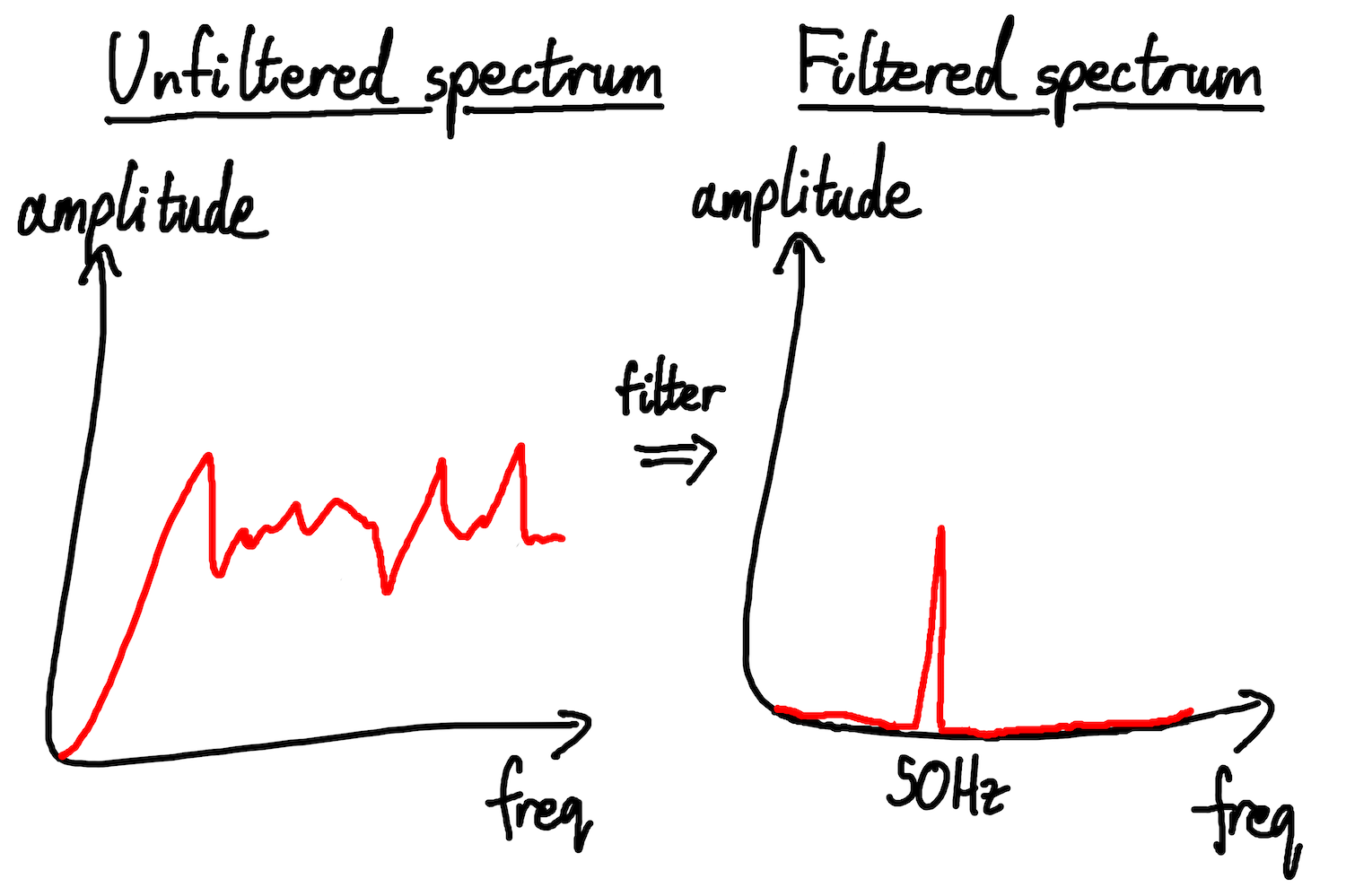
1.2 Filter out frequencies outside of a narrow band around the nominal ENF
A grid’s ENF varies around its nominal value, but not by much. In historical data for Britain’s 50Hz grid I’ve seen values between about 49.8Hz and 50.2Hz, although fluctuations in other grids may be larger or smaller. We don’t use frequencies outside this range in our analysis, so we filter them out in order to enhance and simplify the rest of our work.
Fig: how applying a filter to a wave affects the frequency spectrum
To remove all but a specified band of frequencies from a clip, we pass the clip through a function called a bandpass filter. Different flavours of bandpass filter cut and preserve frequencies in slightly different ways. They don’t completely remove frequencies outside their band, and they may slightly alter frequencies within it. We can accept some blemishes, but the more precise our filter, the more accurate our results. I chose a type of bandpass filter called a “Butterworth Filter” because it’s designed to disturb the frequencies within the band (the part of the sound that we care about) as little as possible. I chose a filter order of 10, which is quite high, because the higher the order, the sharper the cutoff at the boundaries.
Passing our target clip through a filter produces another clip that contains only frequencies within a narrow range around the nominal ENF. Now we’re ready to extract the true ENF as it varies throughout our recording.
1.3 Estimate the ENF for each second
In order to extract the ENF and its variations from our filtered signal, we need to determine the dominant hum frequency at each second. This value will be our estimate for the ENF at that second. To do this, for each second we need to:
Calculate the amplitude of all frequencies in the signal (a frequency spectrum)
Find the highest amplitude frequency in this spectrum
1.3.1 Calculate the amplitude of all frequencies in the signal
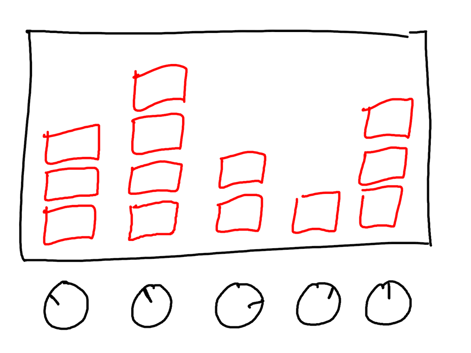
An equaliser (EQ) display on a hi-fi or mixing desk shows the amplitude of different frequencies on a track. It shows how much bass, mid, and high-end are in a sound.
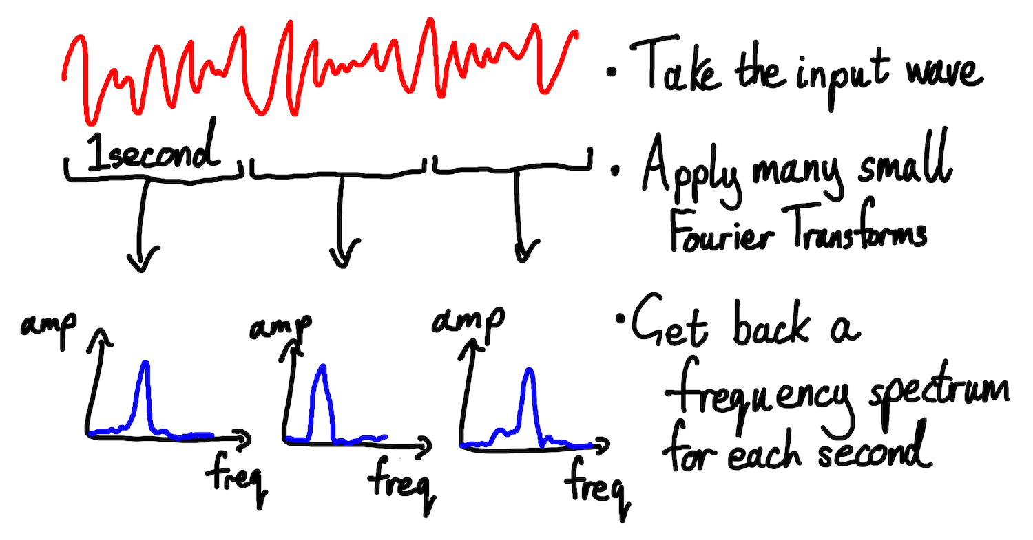
Frequency spectra like those on an EQ are calculated using a family of mathematical processes called Fourier Transforms. To calculate how our clip’s spectrum varies over time, we’ll use a variant called a Short-time Fourier Transform (STFT).
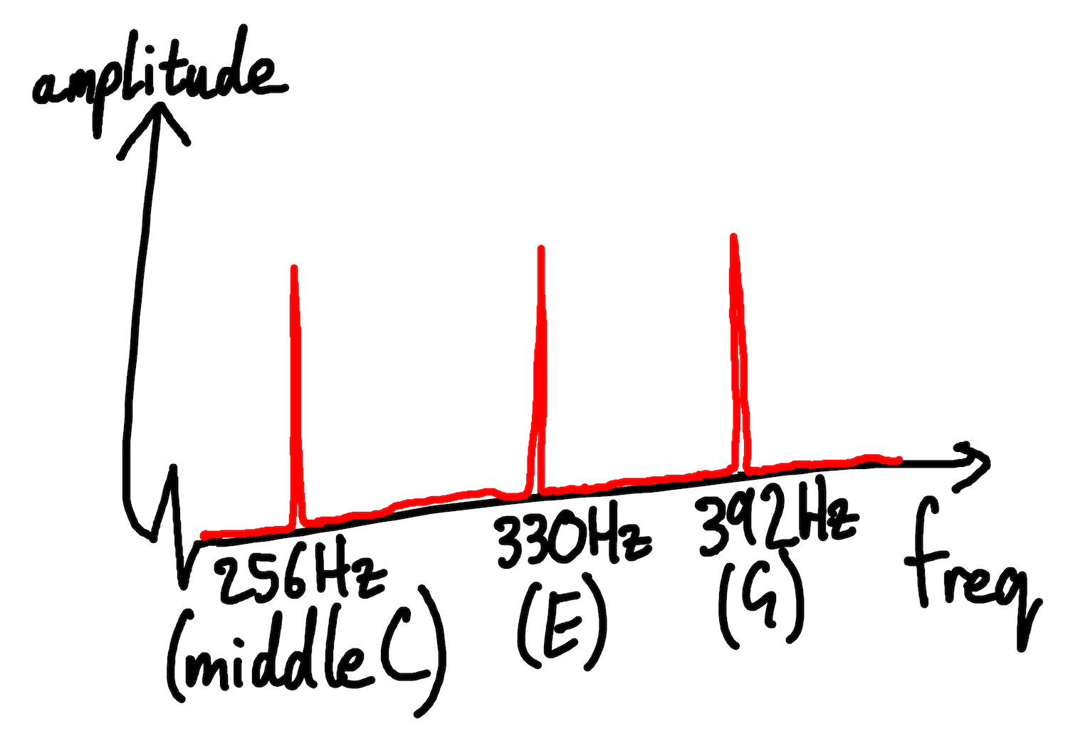
A vanilla Fourier Transform tells us how much of each frequency a wave contains. If we ran a Fourier Transform on a clip of someone playing a C major chord (C-E-G), we would expect it to contain 3 peaks at the frequencies of C, E, and G (ignoring harmonics and other colourations of the sound).
Fig: a Fourier Transform of a C Major chord
A vanilla Fourier Transform performs this decomposition once, for all of a wave. However, we don’t want a single spectrum representing our whole clip. Instead, we want to know how our clip’s frequency content changes over time. An STFT achieves this using multiple, smaller Fourier Transforms. It divides the signal into small time buckets, and performs a separate transform on the portion of the signal in each bucket. It outputs one spectra for each bucket, instead of a single spectra for the whole wave.
Fig: summary of a Short-Time Fourier Transform
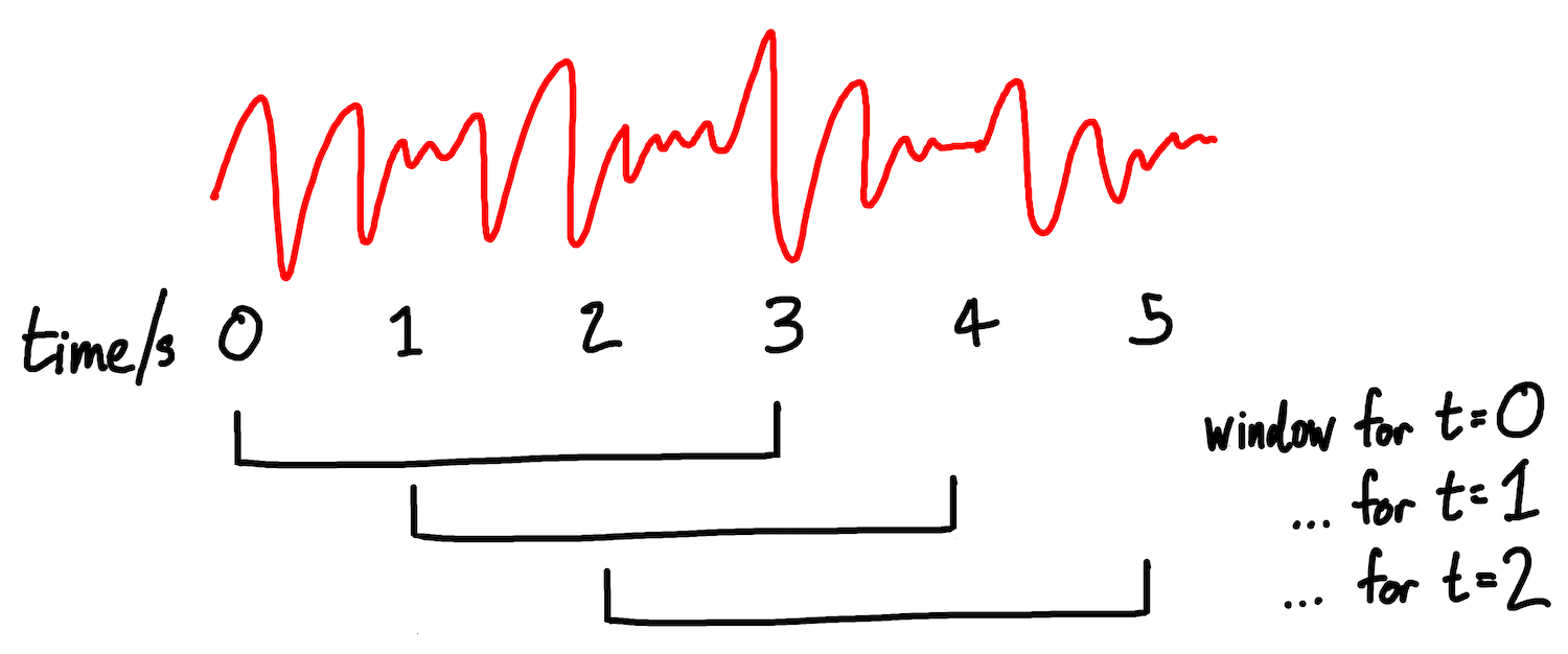
This isn’t quite true - STFT doesn’t process each bucket in isolation. Instead, it uses a sliding window, performing the Fourier Transform on a window that covers both the target bucket and several of its adjacent buckets. It then shifts the window one step along in order to analyse the next target bucket. The caller of the STFT can specify how wide the window should be. This windowing has the effect of smoothing the transitions between each spectrum.
Fig: how an STFT uses a sliding window (of width 3s in this example) to select the portion of the wave to analyse for a given timestamp
In ENF analysis we need to obtain a frequency spectrum for each second, so we use a bucket width of one second. For window size, Hua et al 2017 asserts that 8 or 16 buckets gives the best results.
Note that each value in a Fourier Transform has two components (represented as a complex number) to indicate the phase of the oscillations at that frequency. We don’t need this information (and we don’t need to worry about what it means), so we turn the two components into a single value by taking their combined amplitude.
An STFT gives us an estimate of the frequency spectrum for each second. We expect it to only find frequencies within, or at least very close to, the range of our bandpass filter (say, 49.8Hz - 50.2Hz), because our filter should have removed all other frequencies.
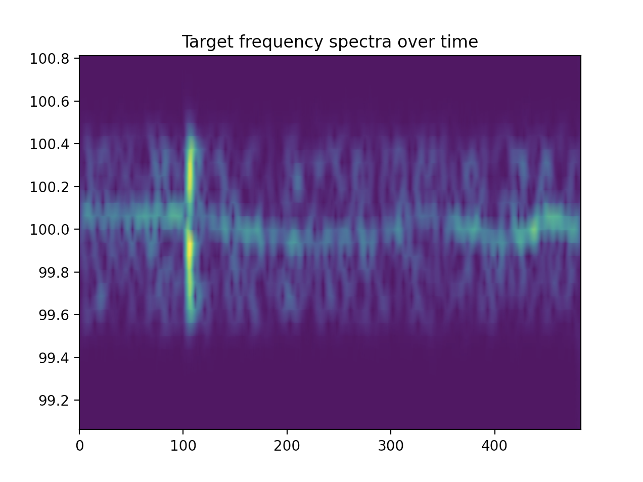
Fig: spectra over time from a target recording. Taken from the first harmonic, hence the y-axis is around 100Hz instead of 50Hz
We can now find the highest amplitude frequency in each second’s spectrum. This gives us the single frequency that we will use as our best guess for the ENF at each second in the recording.
1.3.2 Find the highest amplitude frequency in the spectrum
The simplest estimate for the ENF at a given second would be the frequency in its STFT spectrum with the highest amplitude. However, this would be a small error. This is because we generate our spectra using a discrete STFT, which doesn’t give a continuous output with a value for every possible, arbitrarily precise frequency. Instead, it gives an approximation of a continuous Fourier Transform, represented by a finite number of sampled values. For example, a discrete STFT might return values for the content at 49.800Hz, 49.825Hz, 49.850Hz, and so on, but not for any frequencies between these points.
Fig: a naive estimate of the peak frequency, using the maximum point frequency
It’s unlikely that the true highest amplitude frequency falls exactly on a point that we directly observe. It’s almost certainly somewhere between two of our observations.
Fig: using quadratic interpolation to make a better estimate of the peak frequency
To improve our estimate of the true peak, we use a technique called quadratic interpolation to infer what might be happening between points. We use the values either side of the maximum point to infer the shape that the true, continuous curve takes around this maximum.
You don’t need to know or even read it, but for completeness the quadratic interpolation formula is:
Once we’ve estimated each second’s maximum amplitude frequency, we will have produced a second-by-second estimate of the ENF from our recording, as desired. This estimate can be further improved, for example by combining information from the spectra at multiple harmonics (eg. 50Hz, 100Hz, 150Hz) (Hua et al, 2021), but these improvements are complex and relatively marginal. If implemented they will tweak the values in the ENF series that this step outputs, but won’t affect the rest of the algorithm.
Our target recording has now been turned into an ENF series, one value per second:
[50.225, 50.228, 50.330, 50.227, ...etc...]
Now we need a reference to compare this series against.
3.2 Find a database of reference ENF values from the electrical grid
We need a reference series of true ENF values, taken directly from the grid, every second. These are sometimes published by the grid operator itself (for example, Great Britain’s National Grid), and sometimes by other organisations or individuals (for example, power-grid-frequency.org). In the worst case, it doesn’t seem too hard to record the ENF yourself, although this doesn’t help you if you’re trying to timestamp a historical clip.
The matching process will be faster and more accurate if we can establish a time range in which we know the target recording was taken - for example on a specific day or week - and restrict the reference series to only that period. This limits the amount of reference data that we have to process, and reduces the probability of a spurious false positive.
We download the ENF database and filter it to as tight a date range as we can. We’re now ready for the final step: matching the two series together.
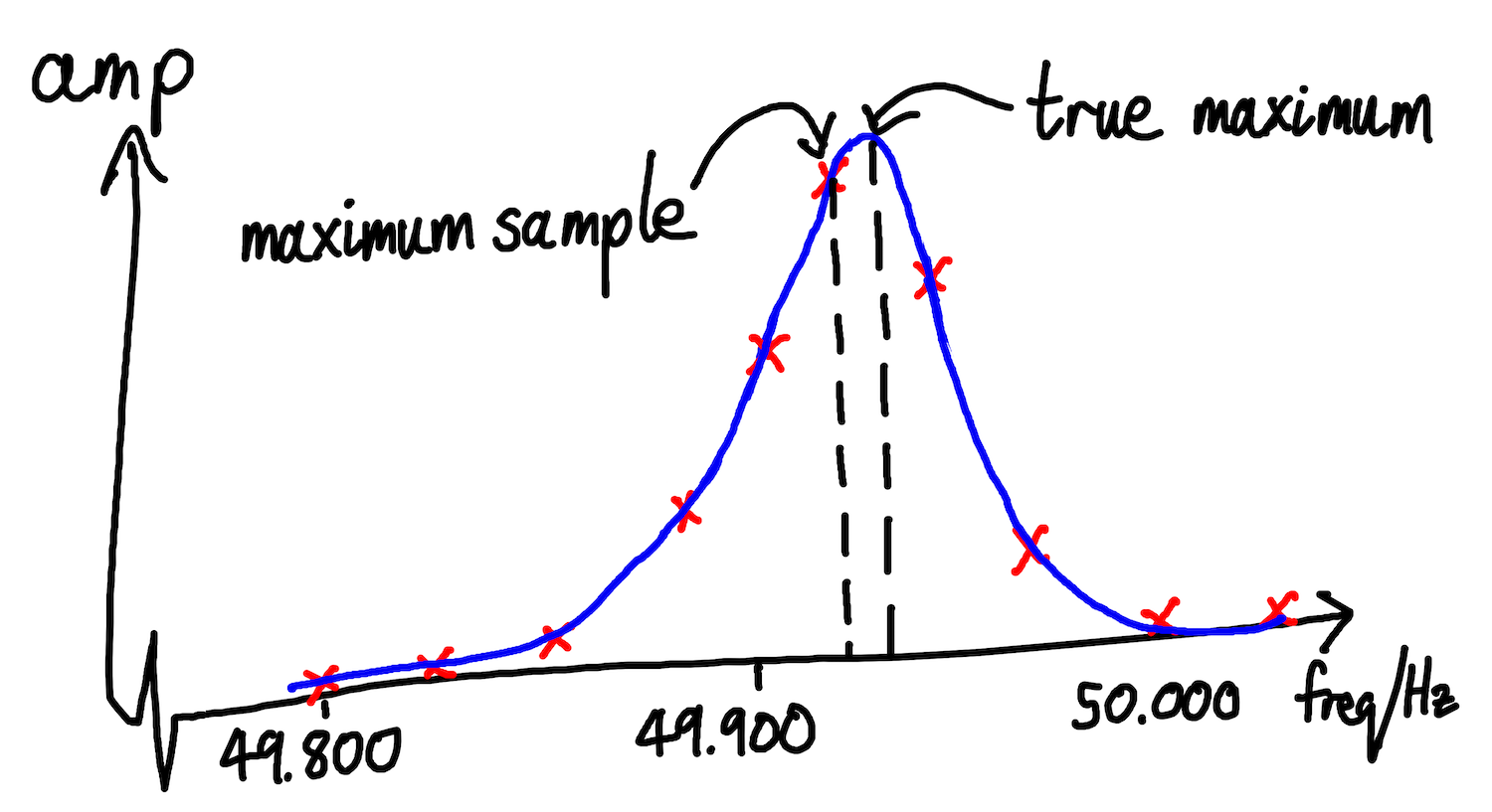
3.3 Match the target ENF series to the reference series
We need to find the section of the reference ENF series that most closely matches the target. This will give us our estimate for the time at which the target recording was made.
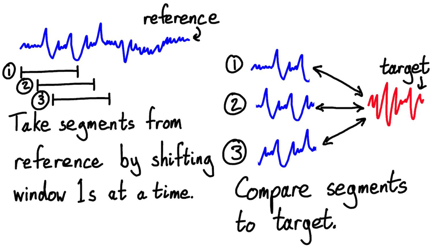
We start by taking a segment from the start of the reference series, of the same length as the whole target series. We compute and record the similarity of the two series (more on which shortly). We then take another segment from the reference, starting one second later, and compute and record the similarity again. We repeat this across the whole reference series.
Fig: taking sliding window-ed segments from a reference series and comparing them to the target series
Once we’ve shifted and compared the target across all points in the reference, we decide which point was the best match. This is then our best guess for the time at which the recording was made.
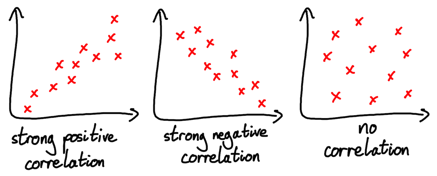
In order to objectively compare the similarity of the target and reference ENFs at different points, we need to be able to numerically measure the similarity between two series. The gauge used in the papers that I’ve read is the Product Moment Correlation Co-Efficient (PMCC). The PMCC is a measure of the linear correlation between two sets of paired data. Do the sets tend to increase and decrease together, inversely, or is there no pattern?
Fig: the basics of correlation
We can pair up the values of the target and reference ENF series from the same offsets, and calculate the PMCC between this paired data. If the target and reference values tend to move up and down in tandem, then this suggests that the target may have been recorded at the same time as the reference. The two series will have a high correlation co-efficient.
Fig: high correlation between target and reference ENFs
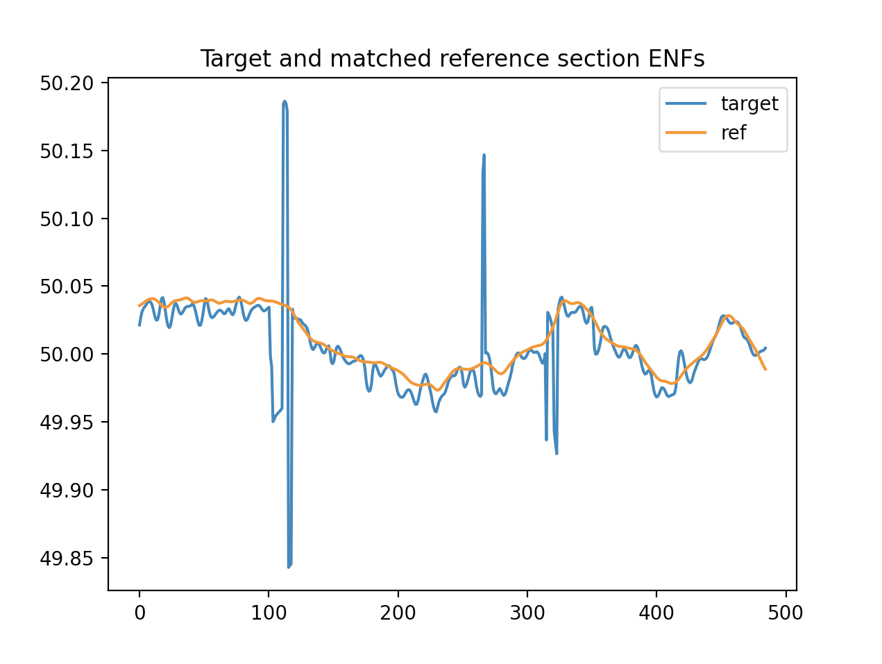
Once we’ve found the section of the reference database that has the highest PMCC with our target recording, we’re done. This is our best guess for when the recording was taken.
Fig: a target series and the best matching section from the reference ENF database
We’ll finish this post with a few finer points.
Finer points
What if there’s no mains hum?
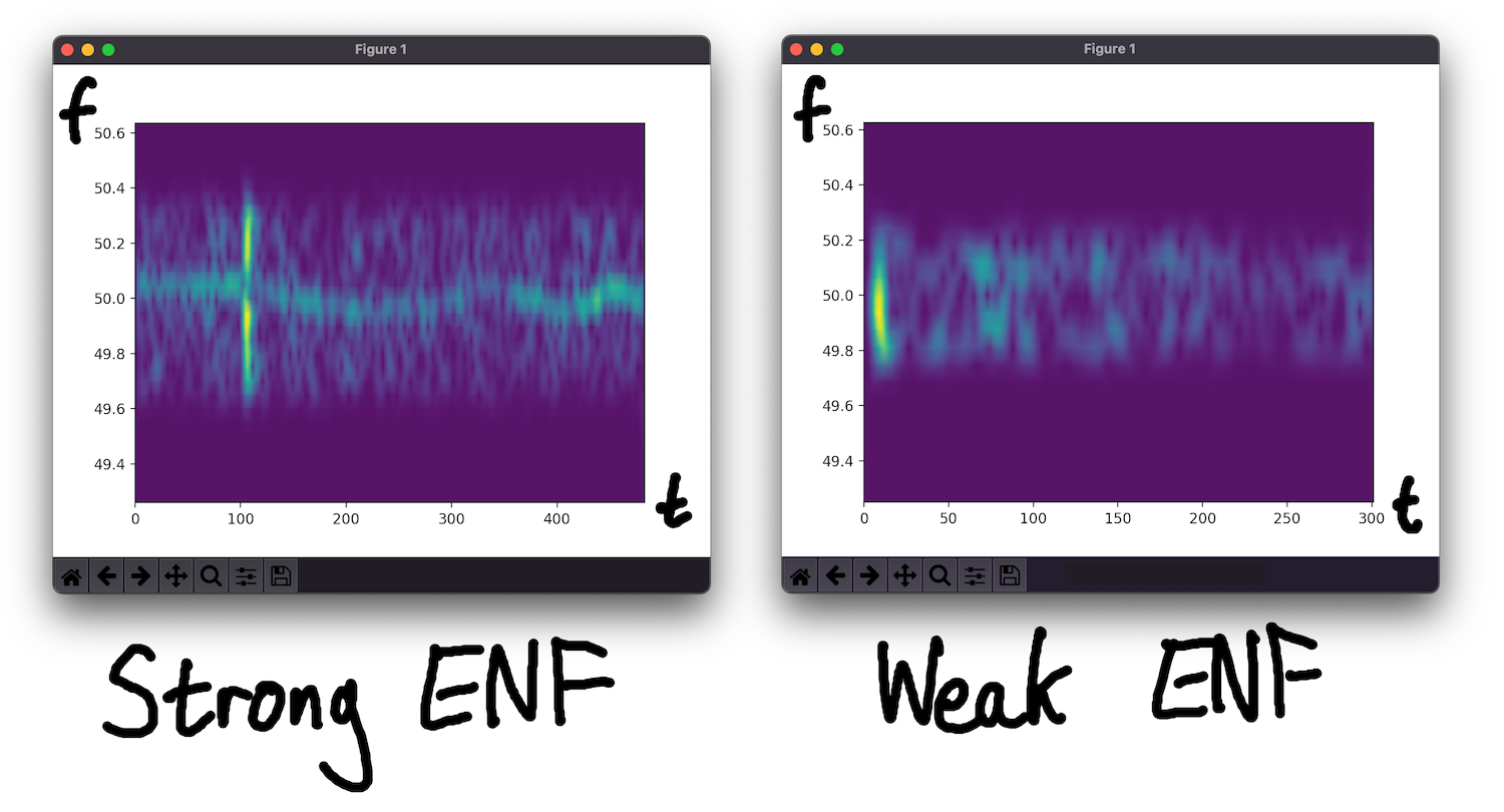
Not all recordings contain a mains hum, perhaps because they weren’t taken near any devices emitting it. If this is the case then we need to abandon our timestamping efforts. The ENF matching algorithm will still produce a guess, even when no real hum is present, and we need to avoid making spurious predictions and assertions based on imaginary correlations. Hua et al 2021 proposes an algorithm to systematically determine whether mains hum is present in a recording, but for an individual case it’s straightforward to manually inspect the output of the ENF extraction step to see whether a pronounced hum is present. The peak in each second’s frequency spectrum should be relatively pronounced, and the ENF should vary slowly, rarely much more than 0.001Hz in a second. Shallow peaks or an erratic ENF suggest that there’s no hum to find.
Fig: a strong ENF trace and a weak one
Using harmonics
Even if a recording is taken in an area where a mains hum is present, the hum may not make its way onto the clip. Some devices deliberately filter out frequencies below 100Hz for the sake of efficiency, as pointed out to me in an email exchange by Guang Hua, the author of many important papers on ENF matching.
However, even if low frequencies are filtered out, we may still be able to detect the hum at higher frequencies. The hum isn’t a single, pure tone. It has a fundamental frequency at 50Hz, but it also has harmonic frequencies at multiples of 50Hz (so 100Hz, 150Hz, 200Hz, etc). This means that if we want to perform ENF matching on a recording containing little-to-no hum at 50Hz, we may instead be able to perform the same analysis on the first harmonic, at 100Hz. If we can extract the harmonic and its variation over time, we can divide each value in the series by two to recover the fundamental ENF.
This is much better than nothing, but these higher frequencies are more vulnerable to noise from other elements on the recording. For example, a typical adult man’s voice contains frequencies between 85-155Hz, which overlaps with the first (100Hz) and second (150Hz) ENF harmonics. The more sounds that overlap with the hum frequencies, the harder it is to distinguish the hum. By contrast, the lower, fundamental frequency range around 50Hz is comparatively unused, and so is likely to be less affected by other elements on the clip. To attempt to get the best of all worlds, Hua et al, 2021 suggests a way to combine harmonics and the fundamental frequency to produce more accurate ENF estimates. I haven’t looked into this approach in detail yet.
Are sub-second offsets a problem?
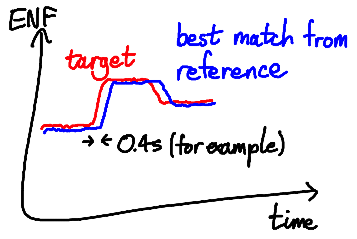
Recordings will almost certainly never start on an exact second. They’ll almost certainly start part way through a second, and so the second-by-second ENF values from the target recording will be taken at a constant, sub-second offset from the reference.
Fig: how a target series can be a fraction of a second displaced from the best match in the reference
Fortunately, our algorithm is not significantly affected by this small shift. The ENF varies slowly, and so its value at t will almost always be very similar to its value at t+1. That means that if a target and reference ENF series are highly correlated, they’ll still be highly correlated when shifted by half a second. Indeed, when the algorithm gives its best guess as time T, it often gives its next best guesses as T+1 and T-1.
In conclusion
ENF matching shows how easy it is to leak information via unexpected side-channels. But despite its intellectual attraction, it might not actually be very important very often. Recordings don’t always contain the right kind of electrical noise. Perhaps they weren’t taken near enough to a source of mains hum, or perhaps the recording device didn’t pick up the right frequencies. In my testing I’ve been able to reliably extract and match the ENF from other people’s example recordings, but not yet from my own. Even if a recording does contain the hum, it needs to be at least 10 minutes long in order to be date-able, and even then the matching process remains prone to false positives.
Even when it works, it’s not clear how much real-world usage ENF matching sees. Trial lawyers probably prefer not to explain signal processing to a jury unless they have no other choice, and the 2012 trial described at the start of this post is the only practical application that I’ve been able to find. Intelligence agencies and police forces might be using ENF matching behind the scenes, but I haven’t been able to find any evidence of this.
If ENF evidence did become widely known and used then it would be straightforward for a knowledgable adversary to manipulate it. The adversary could filter out ENF frequencies from their recordings, making them impossible to timestamp, or even add fake ENF fluctuations to make it look as though a recording was taken at a spoofed time. If prosecution teams keep building cases on ENF analysis, defendants could start claiming that the police doctored not only the content, but the electrical noise too.
This said, almost any kind of evidence can theoretically be faked, and ENF matching can still contribute to the balance of probabilities. It does often work, and researchers are working on improving the technique; some are attempting to use ENF matching principles to deduce the recording time of silent video footage by inferring variations in ENF using the imperceptible flicker of ceiling lights instead of audio hum. ENF matching is amusing and appealing, and whilst half of me isn’t sure if another spigot of leaky metadata is a good thing, the other half hopes that it’s useful somewhere. If you’d like to try out ENF matching for yourself, take a look at my code.
Many thanks to Guang Hua for patiently answering many of my questions about ENF matching.